8 Running and Interpreting Multiple Regression in JASP

Download Data Sets:

• JASP Data File Regression
• CSV Data File Regression

Now that we have the basics down, let’s add additional predictors used in Li and colleagues (2021) original model to conduct a multiple regression. To do this, we will be conducting a multiple regression to examine how and if Cultural Intelligence, Organizational Culture Differences, and Knowledge Sharing have an impact on our dependent variable, Sustainable Innovation Behavior. Why are we adding additional variables? Most of the time our outcomes are affected by more than just one thing, so we can be more accurate in predicting if we include more than one factor that may be relevant. Organizational Culture Differences refers to a company’s corporate culture and measures three aspects: values, systems, and management behaviors. Knowledge Sharing refers to an individual’s willingness to share their cultural knowledge with others in the organization.

The researchers measured Organizational Culture Behavior (OCB) by asking participants to answer 5 questions rated on a 7-point Likert scale. Higher scores on this scale indicate higher levels of Organizational Culture Behavior. A sample item includes, “Organizations uses consensus seeking rather than authoritarian decision making.”

The researchers measured Knowledge Sharing (KS) by asking participants to answer 4 questions rated on a 7-point Likert scale. Higher scores on this scale indicate higher levels of Knowledge Sharinh. A sample item includes, “The more knowledgeable members will provide the other members with knowledge or skills that are difficult to acquire for free.”

Hypotheses

Our hypothesis concerns whether we can predict Sustainable Innovation Behavior using three separate predictor variables: Cultural Intelligence, Knowledge Sharing, and Organizational Culture Differences.

The null hypothesis is:

• Conceptual H₀: Cultural Intelligence, Knowledge Sharing, and Organizational Culture Differences will not predict Sustainable Innovation Behavior.
• Mathematical H₀: b = 0

The alternative hypothesis is:

• Conceptual H₁: Cultural Intelligence, Knowledge Sharing, and Organizational Culture Differences will predict Sustainable Innovation Behavior.
• Mathematical H₁: b ≠ 0

Assumption Testing

Let’s walk through testing all six of our assumptions.

Assumption One: Are our variables continuous?

Yes. Our predictors, Cultural Intelligence, Knowledge Sharing, and Organization Culture are all continuous variables measured using multiple item Likert scale questionnaires. Our outcome of Sustainable Innovation Behavior is also continuous.

Assumption Two: Are the variables normally distributed?

To continue our assumption testing, click Descriptives. When the “Descriptive Statistics” window pops up, we will need to move the following study variables to the “Variables” box on the right: Cultural Intelligence, Knowledge Sharing, Organizational Culture Differences, and Sustainable Innovation Behavior.

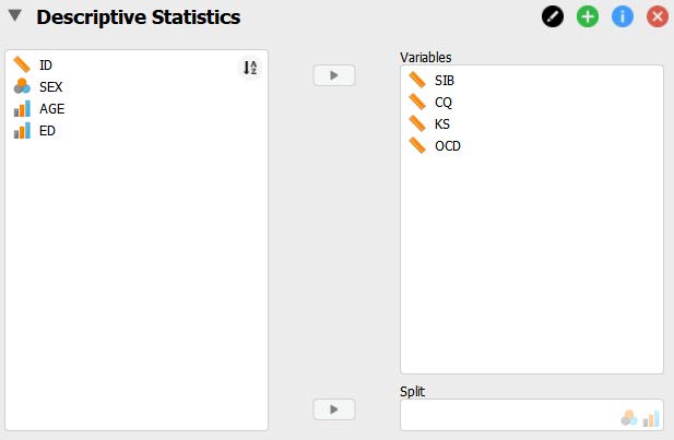
In the Statistics drop down menu, check the boxes next to Skewness and Kurtosis under Distribution.

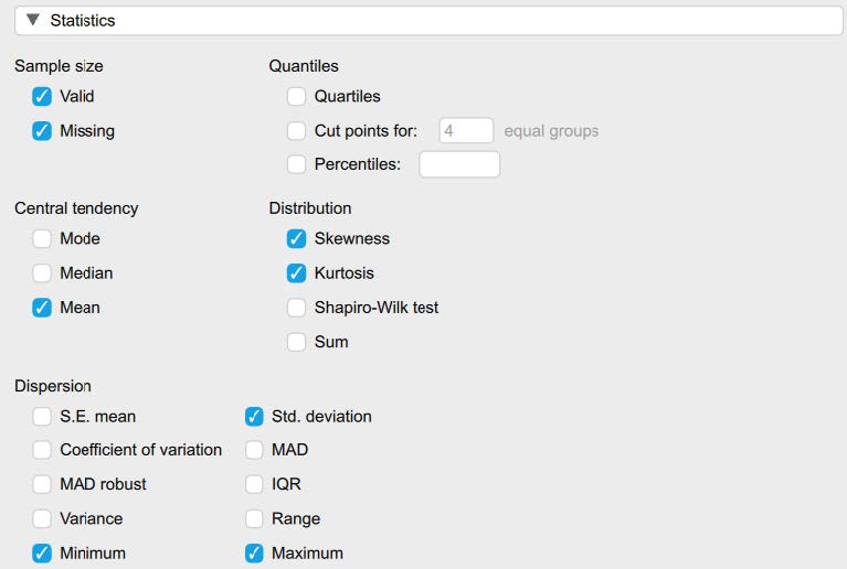
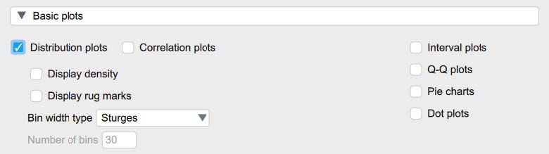
Under Basic Plots select Distribution Plots. In the Plots drop down menu you want to select several options for the next set of assumptions.

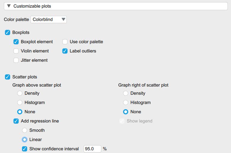
1. Under Boxplots select Label outliers
2. Under Scatterplots
   1. Select None under Graph above scatter plot
   2. Select None under Graph right of scatter plot
   3. Select Add regression line
      1. Under Add regression line select Linear and Show confidence interval 95.0%

Now let’s look at our results. We want histograms that look approximately symmetrical as well as skewness and kurtosis statistics between -2 and +2 for each of our study variables.

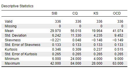
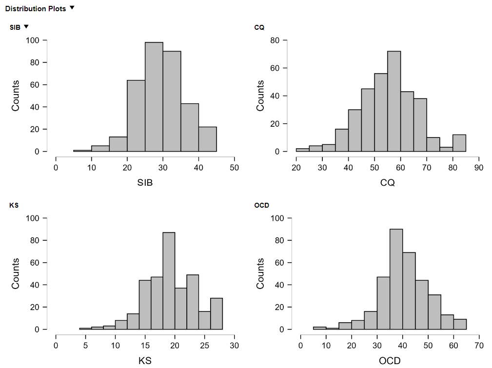
Looking at our results in the preceding images, we see that our skewness and kurtosis values are all within the acceptable range of -2 to +2. Our histograms also confirm that our variables are relatively normally distributed, with approximately symmetrical distributions; however, as we pointed out with the simple regression, the way the histograms for each of the variables have a slight tail to the left indicates we may have outliers present in the bottom quartiles of these distributions. To confirm, let’s move to our next assumption.

To report these results in APA format, we can write:

The scores on all four of our study variables were normally distributed, with skewness and kurtosis statistics within the acceptable range of -2 and +2.

Assumption Three: Are there any outliers?

To determine if there are any outliers within any of our study variables, we will look at the boxplot output in the following image. As suspected from the preceding histograms, there are outliers present in the bottom quartiles of each of the four variables. There are two outliers in the Sustainable Innovative Behaviors variable, two outliers present in the Cultural Intelligence variable, one outlier in the Knowledge Sharing variable, and several outliers present in the Organizational Cultural Differences variable.

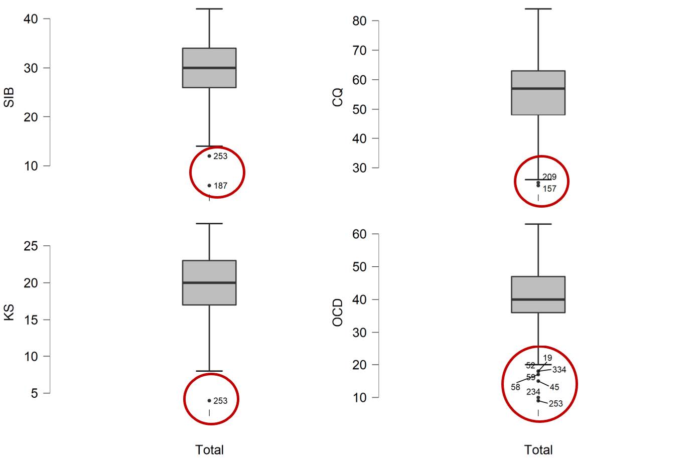
To report this using APA format, we would write:

There were outliers identified across all four study variables in the bottom quartile of the distributions. There were two outliers in the Sustainable Innovation Behavior distribution, two outliers present in the Cultural Intelligence distribution, one outlier in the Knowledge Sharing distribution, and several outliers present in the Organizational Culture Differences distribution.

Assumption Four: Are the relationships of interest linear?

Now we need to look at the scatterplots we requested in our output. Looking at our scatterplots, all of our predictors (Cultural Intelligence, Knowledge Sharing, and Organizational Culture Differences) seem to have a linear relationship with our outcome variable, Sustainable Innovation Behavior.

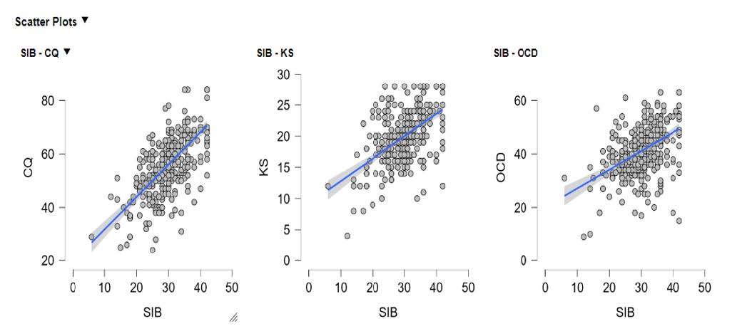
Assumption Five: Are there concerns with heteroscedasticity?

Again, looking at our scatterplots, there is not a big concern for any cone-shaped distributions. Though there is certainly variability along our best-fit line, there is not one area of the line that has drastically different levels of variability than another. In other words, our error variances or residuals seem to be relatively similar across all values of our predictors.

Related, we will also take a closer look at our residuals to see if they are normally distributed when we get to our actual regression analysis and output.

Assumption Six: (For the multiple regression only) Are our predictor variables highly correlated?

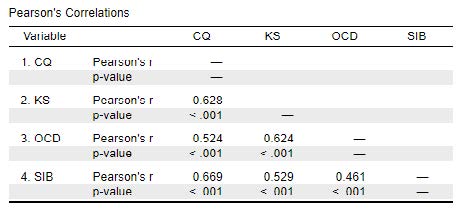
If our predictor variables are highly correlated with each other, this can create problems in interpreting the results of the analysis. Collinearity is the term used to describe this issue of high correlation between predictor variables. One way to check for collinearity is by looking at the correlations between the variables. Another method is by checking the Variance Inflation Factor (VIF) and Tolerance statistics. Let’s begin by using what we learned in the correlation exercise, let’s click the regression menu, select correlation, and then select our four variables. We are interested in looking at the Pearson’s r values for our study variables, so we won’t select any fancy options this time.

In our output table, we see that all three predictors are related to our outcome. We will consider those relationships in more detail with our actual regression analysis. For now, we are concerned with whether our three predictors are too highly correlated. In this case, the Cultural Intelligence and Knowledge Sharing are correlated at .63, meaning that the more cultural intelligence, the more knowledge sharing there is. This correlation is strong, so it is high enough that we may be concerned about multicollinearity in our data. Cultural Intelligence and Organization Culture Difference are moderately correlated at .52 and Knowledge Sharing and Organization Culture Difference are also highly correlated at .62. Keep in mind, we will also look at the VIF and tolerance values in the regression output as additional information about this assumption.

Primary Analyses

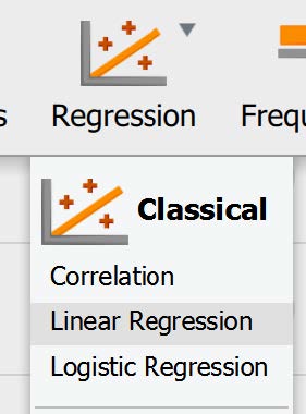
Now we are ready to run our multiple regression model. We will go back up to the regression tab at the top of the JASP menu bar and select the option for linear regression.

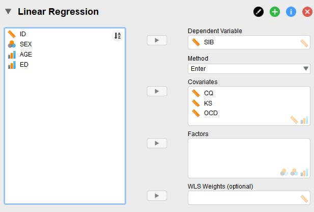
In the main regression menu, we will move over Sustainable Innovation Behavior as our dependent variable and Cultural Intelligence (CQ), Knowledge Sharing (KS), and Organizational Culture Differences (OCD) as our covariates (or predictor variables).

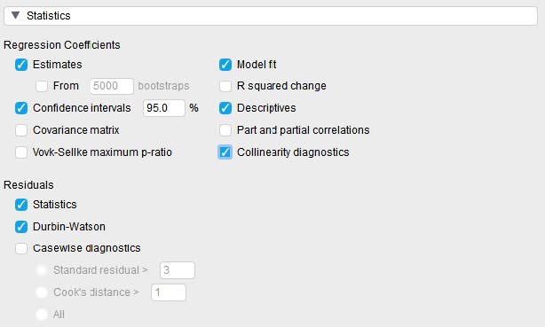
There is nothing we need to adjust in the “model” drop down, so we will move on to “statistics”. In addition to the default settings, we will click:

• “Confidence intervals” under regression coefficients to get a range of likely slope values.
• “Statistics” under residuals to look at the typical amount of error in our model.
• “Descriptives” in the right column of options, just to look at typical values in our dataset.
• “Collinearity diagnostics” to continuing checking assumption six, that we do not have multicollinearity.
• “Durbin-Watson” to check assumption seven, that we have independence of errors.

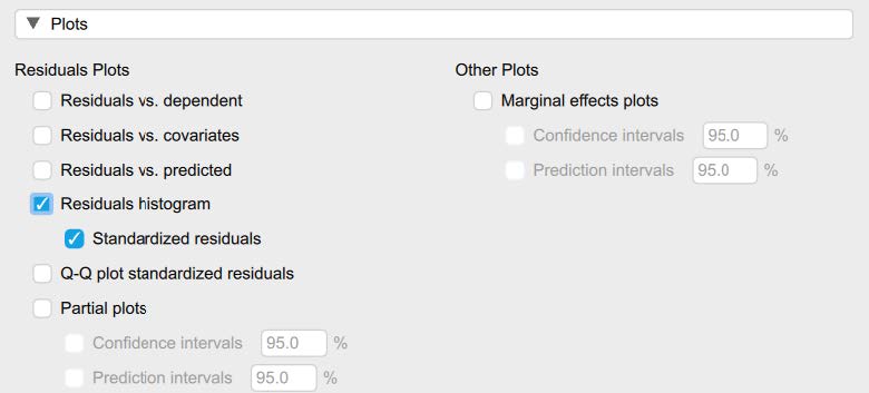
We will also skip over the model specification dropdown and move onto plots. In the plot dropdown, we will click on Residuals vs. histogram to request residuals plotted as a histogram.

Now we’re ready to look at our output! First let’s begin by checking our remaining assumptions.

Assumption Six: Are our predictor variables highly correlated?

As mentioned previously, if our predictor variables are highly correlated with each other, this can create problems in interpreting the results of the analysis. Collinearity is the term used to describe this issue of high correlation between predictor variables. One way to check for collinearity is by looking at the correlations between the variables. Another method is by checking the Variance Inflation Factor (VIF) and Tolerance statistics. The VIF measures how much of the variance in our model is increased due to collinearity (or correlation) between our predictor variables. The Tolerance statistic is the reciprocal of the VIF and measures the proportion of variation in one predictor variable that is not explained by the other predictor variables in the model. In general, we want to see VIF values below 5 and Tolerance statistics above 0.2. If the VIF values are higher than 5, it suggests that there may be too much collinearity between the predictor variables, and this can lead to inaccurate estimates of the regression coefficients. In other words, it can be difficult to determine which predictor variables are contributing to the outcome variable. If our VIF values are above 5, we may need to: (1) remove one or more predictor variables or (2) combine variables into composite scores.

Assumption Seven: Do we have independence of errors?

One important consideration in regression analysis is whether the residuals (the differences between the actual values and predicted values) are correlated with each other or not. The Durbin-Watson statistic is a measure of this correlation. When the Durbin-Watson statistic is between 1.5 and 2.5, it suggests that there is not a significant correlation between the residuals or errors in our model. This is important because if there is a high degree of correlation between residuals, it can suggest that the model is not capturing all the relevant information about the relationship between the variables. In other words, the model may not be a good fit for the data. A Durbin-Watson statistic outside of the 1.5-2.5 range may indicate that there is a problem with the model, and further investigation may be needed to determine the cause of the correlation between residuals.

The Durbin-Watson statistic is a part of the Model Summary results. If this value is between 1.5-2.5, we are not concerned there is a significant amount of correlation between the residuals.

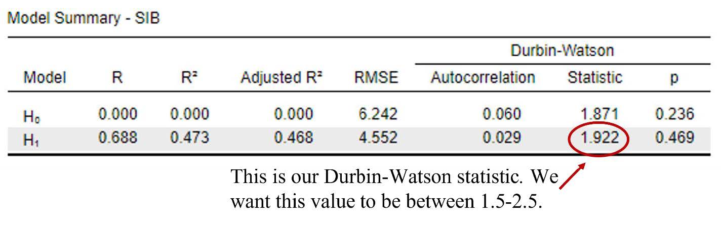
Looking at the preceding figure, we can determine that our Durbin-Watson statistic is within the acceptable range of 1.5-2.5. To report this in APA format:

The model has acceptable independence of errors, Durbin-Watson = 1.92.

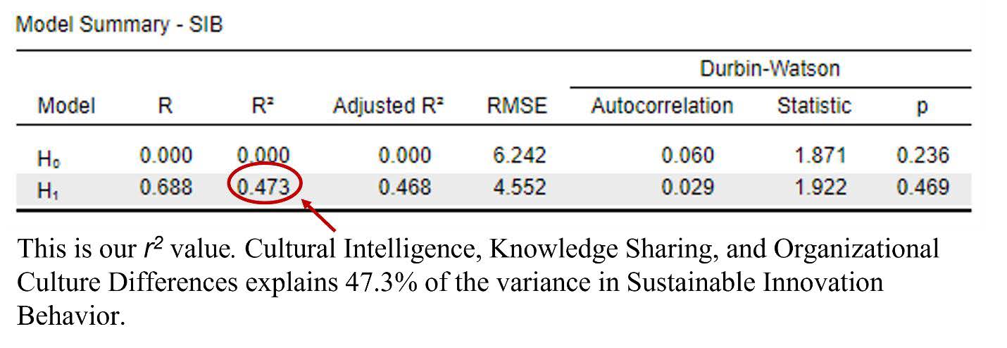
Let’s look at our new output with three predictors. In the Model Summary table, we see that our three variables together are correlated with Sustainable Innovation Behavior at .688 (Multiple R). We also see that, together, Cultural Intelligence, Knowledge Sharing, and Organizational Culture Differences explain 46.8% (R²) of the Sustainable Innovation Behavior. That number grew from 44.8% in our simple regression with only Cultural Intelligence. That tells us that Knowledge Sharing and Organizational Culture Differences do help explain a little bit more about Sustainable Innovation Behavior, but only about 2% more when we add all three predictors together.

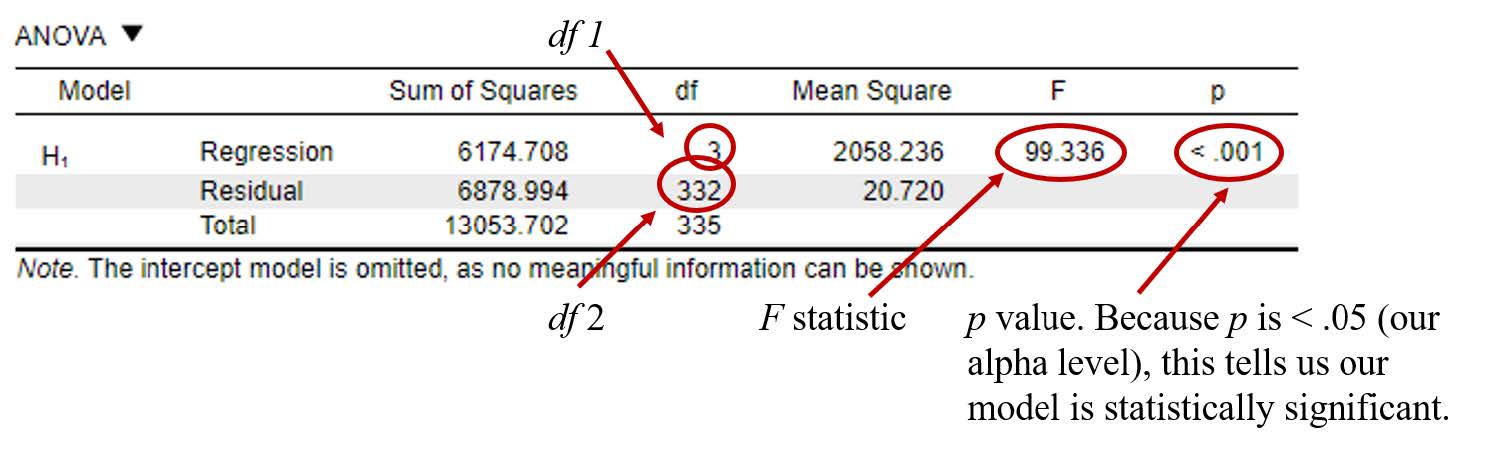
Our ANOVA table shows us that our linear model, including the three predictors, is explaining a significant amount of variance in Sustainable Innovation Behavior. The F value of 99.36 has a p value less than .001, which is below our .05 cutoff. This tells us that our overall model is significant.

Now that we have determined that we have a significant overall model predicting Sustainable Innovation Behavior in the workplace, we would like to gain a better understanding of the relationship between each of our predictor variables with the dependent variable. To do this, we are doing to look at the slopes of each of our predictors, which we’ll find in the coefficients table. Our intercept now reflects if you are zero on all three predictors. So, we can say if a person has no Cultural Intelligence, no Knowledge Sharing, and no Organizational Culture Differences, the average Sustainable Innovation Behavior is 6.91. The slope for Cultural Intelligence has gotten smaller now. That’s because Knowledge Sharing and Organizational Culture Differences are explaining some of the variance now too, making the effect of Cultural Intelligence a bit weaker. The slope of Cultural Intelligence accounting for Knowledge Sharing and Organizational Culture Differences, is .294. Our associated t value of 10.187 has a p value of <.001, which is less than .05. We would say that Cultural Intelligence is a significant predictor of Sustainable Innovation Behavior when you also account for Knowledge Sharing and Organizational Culture Differences. Knowledge Sharing does have a significant slope (b = .196, t = 2.322, p < .02). For every one-unit increase in Knowledge Sharing, you can expect Sustainable Innovation Behavior to increase by .196. Organizational Culture Differences does not have a significant slope (b = .065, t = 1.881, p = .06). For every one-unit increase in Organizational Culture Differences, you can expect Sustainable Innovation Behavior to increase by .065.

Our standardized slopes further show us that Cultural Intelligence (beta = .53) is a stronger predictor than Knowledge Sharing (beta = .13) and Organizational Culture Differences (beta = .10).

Coefficients table from multiple regression output in JASP.

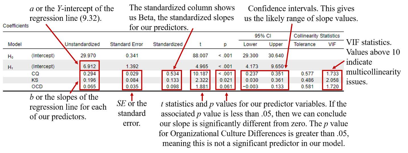
The other piece of information we are interested in is the collinearity statistics in the last two columns. The VIF measures how much of the variance in our model is increased due to collinearity (or correlation) between our predictor variables. The Tolerance statistic is the reciprocal of the VIF and measures the proportion of variation in one predictor variable that is not explained by the other predictor variables in the model. In general, we want to see VIF values below 5 and Tolerance statistics above 0.2. If the VIF values are higher than 5, it suggests that there may be too much collinearity between the predictor variables, and this can lead to inaccurate estimates of the regression coefficients. In other words, it can be difficult to determine which predictor variables are contributing to the outcome variable. If our VIF values are above 5, we may need to: (1) remove one or more predictor variables or (2) combine variables into composite scores.

Our tolerance values range from .49 to .58, meaning that between 49% and 58% of the variance in the predictors is unshared. Our largest VIF value is 2.06, which is below 10, so there is not much concern for multicollinearity.

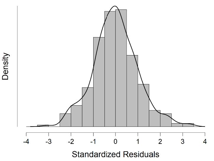
Related to our assumptions, we also want to make sure we take another look at our residuals plot for our multiple regression model. Again, we see that our residuals for our model (based on the regression equation with three predictors) approximate a fairly normal distribution.

Putting it all Together

It’s time to summarize the results of our multiple regression analyses.

Prior to conducting our multiple regression, we tested several assumptions. We examined our predictors (Cultural Intelligence, Knowledge Sharing, and Organizational Culture Differences) and outcome (Sustainable Innovation Behavior) variables for normality and any concerns with outliers. All skewness and kurtosis values were all in the normal range. Upon inspection of variable boxplots and histograms, four outliers were revealed that were retained for analysis. Using a scatterplot, we also visualized the relationships between the variables. Upon viewing the scatterplots, we observed that the relationships appeared linear and that there were no concerns with heteroscedasticity. Plots of the residuals also showed that the residuals were approximately normally distributed. We also looked at the correlation between our predictor variables, finding that the variables were moderately correlated (r range = .52 to .63). The variance inflation factor values for our model were all less than 2.05, providing support that there were not substantial concerns with multicollinearity. The model has acceptable independence of errors, Durbin-Watson = 1.92.

In our multiple regression, we examined how the Cultural Intelligence, Knowledge Sharing, and Organization Culture affected Sustainable Innovation Behavior. We found that together, these three predictors explained a significant amount of variance in Sustainable Innovation Behavior, F (3, 336) = 99.3, p < .001. Together, the predictors explained 46.8% of the variance in Sustainable Innovation Behavior. Organizational Culture Differences, Cultural Intelligence, and Knowledge Sharing were significant predictors of Sustainable Innovation Behavior, when controlling for the other predictors. Knowledge Sharing was positively related to Sustainable Innovation Behavior (b = .20, SE = .08, t (332) = 2.32, p = .02). Cultural Intelligence was also positively related to Sustainable Innovation Behavior (b = .29, SE = .03, t (332) = 10.19, p < .001). Organizational Culture Differences was not a significant predictor of Sustainable Innovation Behavior (b = .07, SE = .04, t (332) = 1.88, p = .06).

Real World Meaning

From this study, we could share that Cultural Intelligence, Knowledge Sharing, and Organization Culture Differences together impact Sustainable Innovation Behavior, but the strongest relationship exists between Sustainable Innovation Behavior and Cultural Intelligence, where the more cultural intelligence someone has, the more likely they are to also engage in sustainable innovation behaviors in the workplace. The same pattern is true with knowledge sharing, that sharing more information is related to more innovation, just not as strongly as cultural intelligence relates to innovation behaviors. Together, Cultural Intelligence, Knowledge Sharing, and Organizational Culture Differences can explain over half of the variance in Sustainable Innovation Behavior across a sample of individuals in organizations.

In their study, Li et al. (2021) found similar results. They examined how Cultural Intelligence impacted Sustainable Innovation Behavior with Knowledge Sharing as an intermediary variable and Organizational Culture Differences as a moderator. Their results showed that Cultural Intelligence positively impacts Sustainable Innovation Behavior, but this relationship is mediated or linked by Knowledge Sharing. They also found that Organizational Culture Differences did not significantly moderate or change the relationship between Cultural Intelligence and Sustainable Innovation Behavior, but it did impact the relationship between Cultural Intelligence and Knowledge Sharing.

The results of our statistical analysis and that of Li et al. (2021) both suggest that Organizational Culture Differences does not really have a significant impact on our main variable, Sustainable Innovation Behavior. It can also be said that Sustainable Innovation Behavior and Cultural Intelligence do have a strong relationship together whereas the relationship between Sustainable Innovation Behavior and Knowledge Sharing is not as strong.

References

Gölgeci, I., Swiatowiec-Szczepanska, J., & Raczkowski, K. (2017). How does cultural intelligence influence the relationships between potential and realised absorptive capacity and innovativeness? Evidence from Poland. Technology Analysis & Strategic Management, 29(8), 857–871. https://doi.org/10.1080/09537325.2016.1245858

Hu, S., Gu, J., Liu, H. & Huang, Q. (2017). The moderating role of social media usage in the relationship among multicultural experiences, cultural intelligence, and individual creativity. Information Technology & People, 30(2), pp. 265-281. https://doi.org/10.1108/ITP-04-2016-0099

Li, J., Wu, N., & Xiong, S. (2021). Sustainable innovation in the context of organizational cultural diversity: The role of cultural intelligence and knowledge sharing. PloS One, 16(5), e0250878–e0250878. https://doi.org/10.1371/journal.pone.0250878

Pandey, A. & Charoensukmongkol, P. (2019). Contribution of cultural intelligence to adaptive selling and customer-oriented selling of salespeople at international trade shows: does cultural similarity matter? Journal of Asia Business Studies, 13(1), pp. 79-96. https://doi.org/10.1108/JABS-08-2017-0138

Authors

This guide was written and created by Ruth V. Walker, PhD, Ashlyn A. Moraine, and Kristen J. Black, PhD.

Acknowledgements

We would like to thank Jinlong Li, Na Wu, and Shengxu Xiong for generously publishing their data through PloS One.

Copyright

CC BY-NC-ND: This license allows reusers to copy and distribute the material in any medium or format in unadapted form only, for noncommercial purposes only, and only so long as attribution is given to the creator.