
1 Running and Interpreting an Independent Samples t test in JASP
Kelsey L. Humphrey; Ruth Walker; and Erin N. Prince
Download Data Sets:
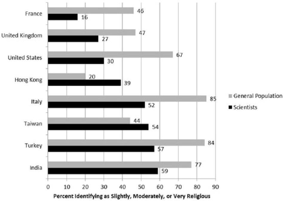
Researchers Elizabeth Barnes, Jasmine Truong, and colleagues (2020) conducted a series of studies at Arizona State University to understand if there is bias against Christian students in the natural sciences. Pew Research Center (2019) surveys have found that approximately 65% of the population in the United States describe themselves as Christian; however, a worldwide sample of over 9,000 scientists in biology and physics found lower levels of religiosity in scientists compared to the general population in the United States (see graph below; Howard Ecklund et al., 2016). Further, 22% of scientists in the United States said that science has made them “much less religious” (p. 5).
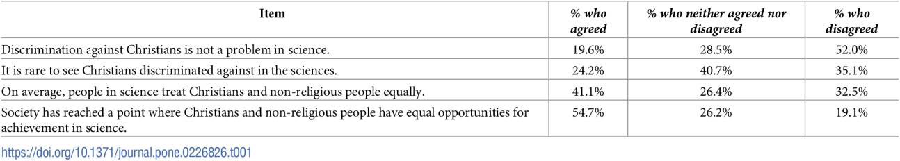
This led Barnes and colleagues (2020) to their research questions: Why are Christians underrepresented in the natural sciences? Do negative stereotypes about the scientific abilities of Christian students put them at a disadvantage in the natural sciences? Their first study found that it was common for biology students to report perceptions of bias against Christians in science (see table below).
Once they gathered data to show that students perceive there is a bias against Christians in science, they wanted to conduct studies to help determine if academic scientists in the natural sciences exhibited biased behavior towards Christian students. To do this, they conducted two experimental studies. We will analyze Study 2 data when we discuss One-Way ANOVAs, for now we will look closer at Study 3. For Study 3, the researchers recruited 261 faculty in biology and randomly assigned them to one of two conditions:
- Faculty in condition one read a graduate student application that signaled evangelism. Their application listed the student taking a mission trip for Campus Crusade for Christ, with a recommendation letter from a mentor in that ministry.
- Faculty in condition two read a graduate student application that listed the student taking a service trip for the United Nations Children’s Fund, with a recommendation letter for a mentor in that organization.
All other aspects of their application were kept consistent (e.g., same GPA and GRE scores). Faculty were asked to rate the student on competence, hireability, and likeability using a 7-point likert scale from 1 (not at all) to 7 (very much). Higher scores on each of these scales indicate higher levels of competence, hireability, and likeability.
Hypotheses
We are going to focus on two of the three outcome variables Barnes and colleagues (2020) measured in their study. Specifically, we will focus on faculty ratings of (1) student competence and (2) student likeability. This means that we will have three different sets of hypotheses.
The null hypotheses are:
- Student Competence
- Conceptual H0: There are no differences in faculty ratings of graduate student competence between the Christian student condition and the Control student condition.
- Mathematical H0: The mean score for graduate student competence in the Christian student condition is equal to the mean score for student competence in the Control student condition; M1 = M2.
- Student Likeability
- Conceptual H0: There are no differences in faculty ratings of graduate student likeability between the Christian student condition and the Control student condition.
- Mathematical H0: The mean score for graduate student competence in the Christian student condition is equal to the mean score for student likeability in the Control student condition; M1 = M2.
The alternative hypotheses are:
- Student Competence
- Conceptual H1: There are significant differences in faculty ratings of graduate student competence between the Christian student condition and the Control student condition.
- Mathematical H1: The mean score for graduate student competence in the Christian student condition is not equal to the mean score for student competence in the Control student condition; M1 ≠ M2.
- Student Likeability
- Conceptual H2: There are significant differences in faculty ratings of graduate student likeability between the Christian student condition and the Control student condition.
- Mathematical H2: The mean score for graduate student competence in the Christian student condition is not equal to the mean score for student likeability in the Control student condition; M1 ≠ M2.
JASP Analyses
In order to run analyses in JASP, the first thing we need to do is open the data set we will be working with. To do this, open JASP and follow the steps below.
File → Open → Computer → Browse → Pick the Independent t Practice Data (Barnes et al., 2020 Independent Samples t Test Data)
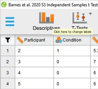
Once the data set is open in JASP, we will change the data labels for our condition variable to make interpretation easier. Currently, the Condition column has either a 0 or a 1 for each participant. To change the numerical data into our categorical labels (i.e., Christian Student or the Control Condition), you will take your cursor and hover over Condition. When you see a note pop up saying, “click here to change labels” click on it.
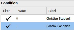
Barne’s et al. (2020) codebook indicate that the appropriate label for 0 is “Christian student” and 1 is “Control condition.” To make this change in our dataset, we will click on the 0 under the Label column and type ‘Christian Student’. Then we will click on the 1 under the Label column and type ‘Control Condition’. After you have changed the labels, you can close the window by clicking on the “x” button.
Assumption Testing
Prior to running our independent samples t test, we first have to check to make sure we meet the assumptions for this statistical test.
Assumption One: Is our independent variable dichotomous and measured at the categorical (i.e., nominal) level?
Yes. Our independent variable for this study is the level of religiosity in the graduate student applications faculty read. Participants either read the scenario featuring a “Christian Student” or a student with no religious affiliation given. This means our independent variable for this particular study is dichotomous (meaning, there are only two categories), and categorical. If you look at the data label icon in JASP, you can see it has the appropriate icon (three overlapping circles) for a nominal/categorical variable. We meet this assumption.
![]()
Assumption Two: Is the dependent variable continuous (i.e., ratio or interval)?
Yes. Our dependent variables for this study are faculty ratings of the graduate student applicants’ likeability and competence. Each variable was assessed using a four-item scale. Faculty rated each item on a 7-point likert scale from 1 (not at all) to 7 (very much). This variable is continuous, meaning it was measured at the interval or ratio level. If you look at the data label icon in JASP, you can see it has the appropriate icon (a ruler) for a scale or continuous variable. We meet this assumption.
![]()
Assumption Three: Are the samples independent?
Yes. Looking at our data set, we can determine that our two groups (Christian Student condition and Control Student condition) are independent. If we look in the “Condition” column, we can see that all biology faculty participants were randomly sorted into either the Christian Student or Control Condition groups – there are no participants who have both labels or any other group value listed. Thus, we can conclude that participants in both groups are independent of one another. No participant is in more than one group. We meet this assumption.
Assumption Four: Is the dependent variable normally distributed for each group of the IV?
To check our data for the next two assumptions, we will use the Descriptive analysis tab. Click Descriptive. When the “Descriptive Statistics” window pops up, we will need to move our dependent variable to the “Variables” box and our independent variable to the “Split” box using the arrows depicted in the photo below – this is so we can examine normality in the DV for both of our groups separately.
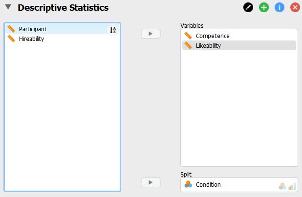
Once we have our variables in the appropriate boxes, we are going to ask JASP to run the various statistics and graphics we will need to interpret for our assumptions by clicking on the appropriate boxes in the test window. We will be asking JASP to provide us with all possible output we may want to look at for our assumptions; however, we will focus on interpreting the output that you will be expected to analyze for your statistical lab assignment.
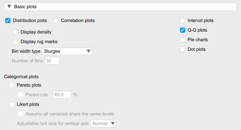
- Under the “Customizable Plots” tab we will check the “Boxplots,” “Boxplot element,” “Jitter element,” and “Label outliers” boxes. We will also check “Distribution plots” and “Q-Q plots” under the “Basic plots” tab.
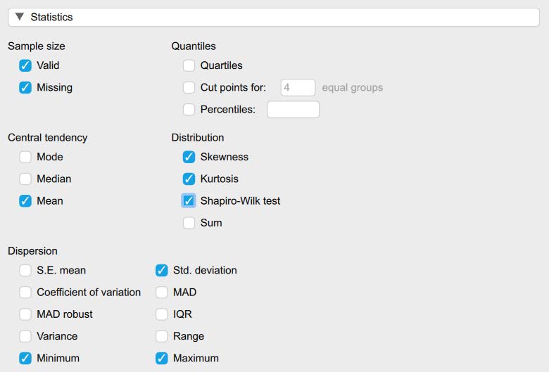
- Under the “Statistics” tab we will check the “Skewness,” “Kurtosis,” and “Shapiro-Wilk test” boxes.
See the image below to make sure your test window has all the appropriate boxes selected.

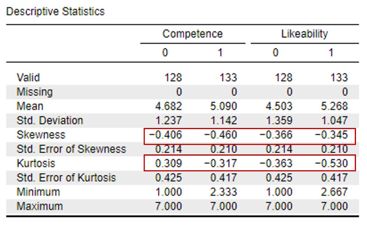
To determine if we have normally distributed data, you can look at the histograms and Q-Q plots to visually inspect the data. For this course, however, we will focus on interpreting the skewness and kurtosis statistics. Specifically, we want skewness and kurtosis statistics that are between -2 and +2. Remember, we have two groups, so we have to check the skewness and kurtosis values for our dependent variable, biased behavior, for both the Christian Student condition and the Control Condition. Looking at the values on the output copied below, we can see our skewness values for competence (-0.41, -0.46) and likeability (-0.37, -0.35) are all within the acceptable range of -2 and +2. Additionally, the kurtosis values for competence (0.31, -0.32) and likeability (-0.36, -0.53) are also within the acceptable range of -2 and +2.
To report these results in APA format, we could write:
Competence and likeability for the Christian Student condition and the Control Condition were normally distributed, skewness and kurtosis statistics were between -2 and +2.
Assumption Five: Are there any outliers in the sample?
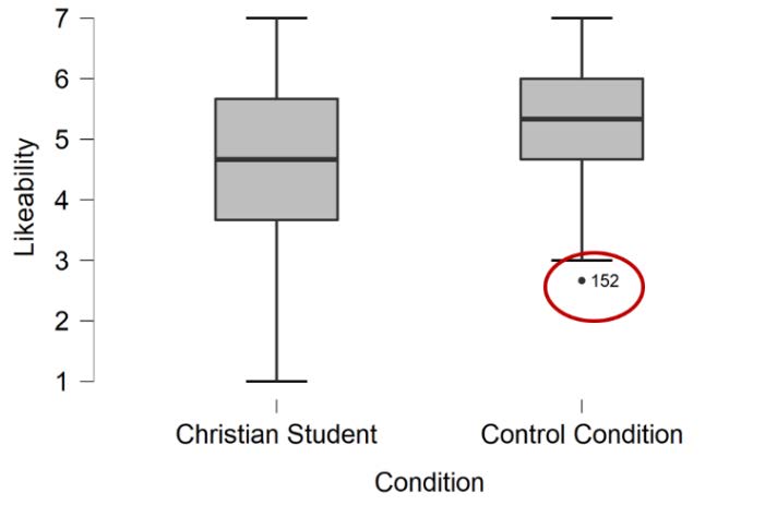
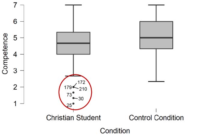
To assess for outliers, we will look at the boxplots in our JASP output. If we have outliers, they would be outside the top and bottom lines or whiskers. You can see we have one outlier identified in the boxplot for likeability for the Control Condition, below the lower quartile. Also, we have 6 outliers in the boxplot for competence for the Christian Student condition, below the lower quartile.
To report this in APA format, we could write
There was one outlier in the boxplot for likeability for the Control Condition and six outliers in the boxplot for the competence for the Christian Student condition, as assessed by the inspection of a boxplot.
As we have discussed previously, when we have outliers we have to decide if they are going to correct it, keep it, delete it, or replace it. Although we did not collect this data personally, the majority of survey research is collected online through programs such as Qualtrics, QuestionPro, and Survey Monkey. Thus, we can assume the outliers for likeability and competence in the Control and Christian Student conditions were not a data entry error. Cleaning data for random responding and fast survey completion times would have occurred in the data cleaning process, before we got to our analyses, so we can rule those out as well. As a researcher, you would then have to decide if the outliers are exerting a significant enough impact on your results to warrant deletion. It is common for researchers to run their analyses with the outliers retained and with the outliers deleted to see if their exclusion changes the results. With either decision, you would need to add those details when you report your results. In this case, we will retain the outliers; however, we will discuss whether the results would be different if they were deleted when we cover the primary analyses.
Assumption Six: Are there homogeneity of variances?
To determine if we have homogeneity of variances, we need to ask JASP to run our independent samples t test. Checking for this assumption is a part of the overall independent samples t test. Let’s move onto our primary analyses below, and complete checking this assumption in that section.
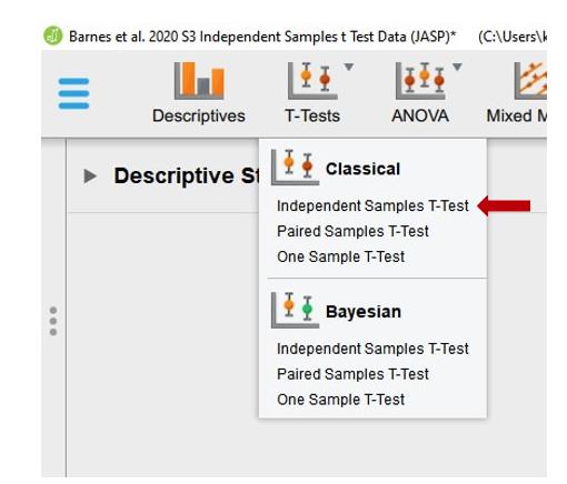
Primary Analyses
To run an independent samples t test, go to T-Tests at the top of the JASP screen and click on Independent Samples T-Test. See the image below.
-
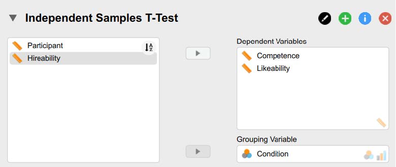
First, we need to move our dependent variables [Competence, Likeability] to the “Variables” box and our independent variable [Condition] to the “Grouping Variable” box. We are then going to ask JASP to run the various analyses we will need to interpret for our test by clicking on the appropriate boxes in the test window.
-
Under “Tests” we will check the “Student” and “Welch” test boxes.
-
Under “Assumption Checks” we will check the “Equality of variances” box.
-
Next, we will check the “Effect Size” box and make sure that “Cohen’s d” is selected.
-
Other options that are helpful to ask JASP to provide you with include the “Descriptives” and “Descriptives Plots.”
See the image below to make sure your test window has all the appropriate boxes selected.
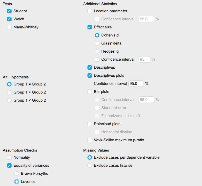
Now that we have asked JASP to run the appropriate analyses, we can begin our interpretation of the results. The first thing we need to do is go back to our last assumption and determine if we meet the assumption for homogeneity of variances.
Are there homogeneity of variances?
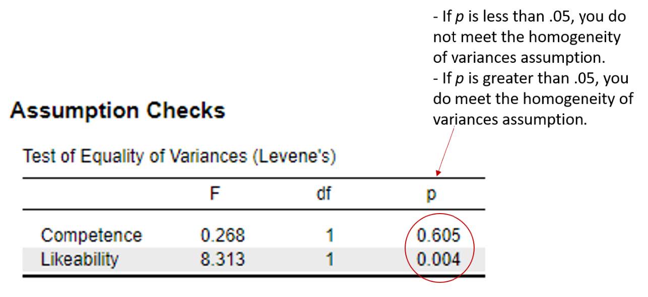
To interpret the results of the Levene’s test, we need to look at the significance or probability value. If p is less than .05, the test is significant, and we do not have homogeneity of variances. If p is greater than .05, the test is non-significant, and we do have homogeneity of variances. We meet this assumption.
- If homogeneity of variances was met, you can proceed with interpreting the “Student” independent samples t test results.
- If homogeneity of variances was violated, you can still continue conducting an independent samples t test, but will you need to interpret the “Welch” independent samples t test results instead. The Welch t test is referred to as the unequal variance t test, separate variances t test, or the Welch t test after its creator (Welch, 1947). This test can handle testing mean differences between samples with unequal variances. To include the Welch test in your results, check the “Welch” box under “Tests.” I often click this box when running an independent samples t test automatically, just in case the Levene’s test is significant and there are not equal variances.
To report the results of the Levene’s test in APA format, it might look something like this:
There was homogeneity of variances, as assessed by the Levene’s test for equality of variances, for competence, p > .05. However, homogeneity of variances was violated for likeability, p < .05.
Interpreting the Statistical Significance of Independent Samples t Tests
The first thing we will interpret is the statistical significance. To do this, we are going to look at the “Independent Samples T-Test” table. Because we have three different dependent variables, we are going to do this one at a time. For our first dependent variable, likeability, we did not meet the assumption of homogeneity of variances. Thus, we are going to interpret the “Welch” t test results in the second row.
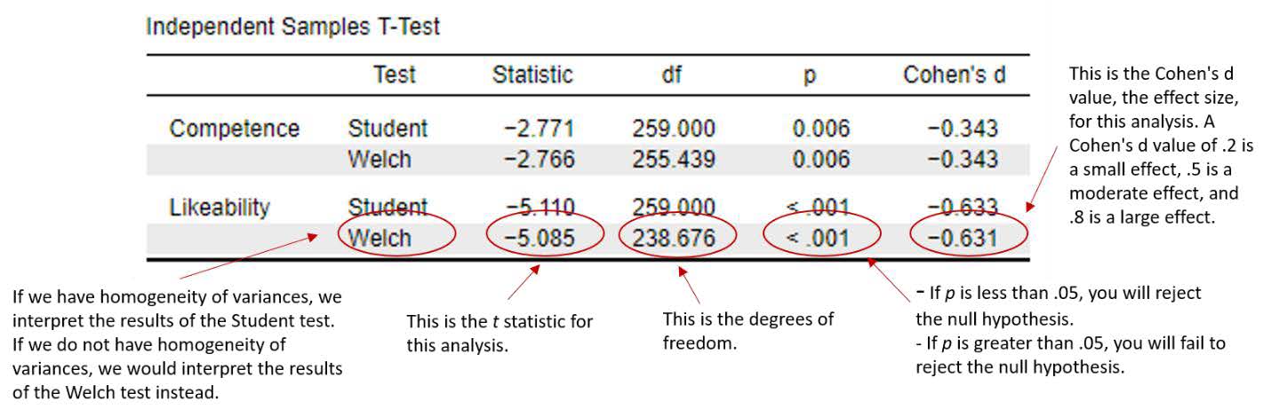
To interpret the results, we want to look at the p value. If p is less than our alpha level of .05, we will reject the null hypothesis. There is a significant statistical difference between the group means. If p is greater than our alpha level of .05, we will fail to reject our null hypothesis. There is not a significant statistical difference between the group means. For our Likeability variable, you can see that our p value is < .001. This is less than our alpha level of .05, so we will reject our null hypothesis. There is a significant statistical difference between the Christian Student condition and the Control Condition on faculty ratings of likeability.
For our second dependent variable, competence, we did meet the assumption of homogeneity of variances. Thus, we are going to interpret the “Student” t test results in the first row. For our Competence variable, you can see that our p value is < .01. This is also less than our alpha level of .05, so we will reject our third null hypothesis. There is a significant statistical difference between the Christian Student condition and the Control Condition on faculty ratings of competence.
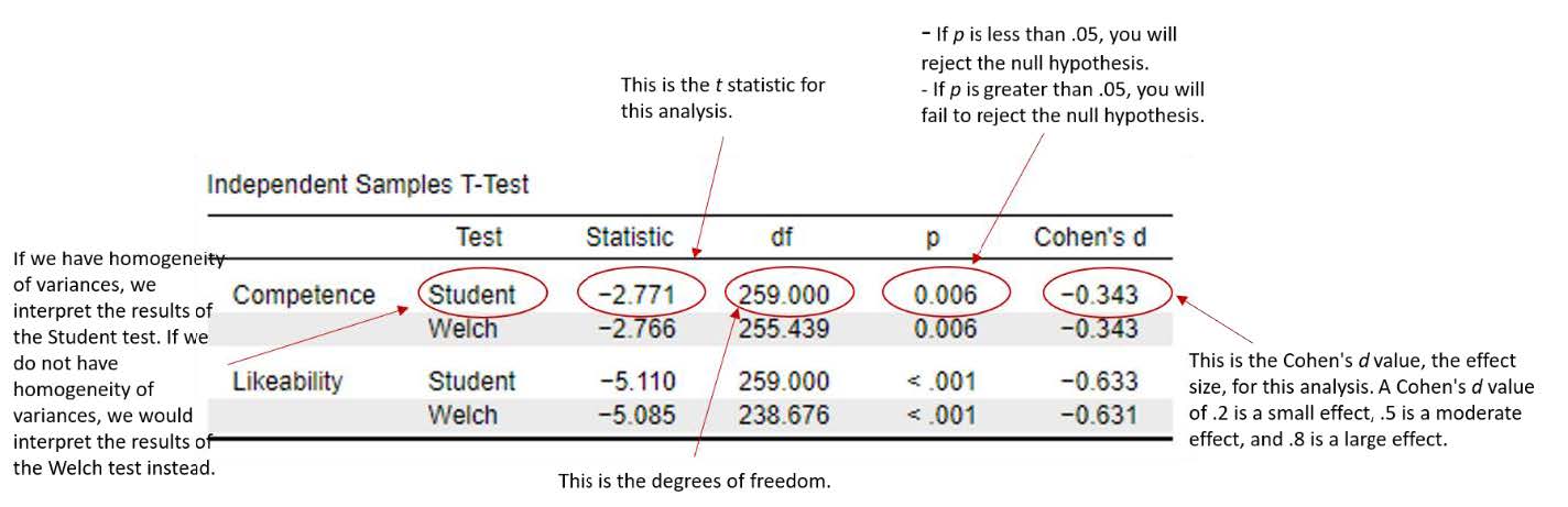
Writing the basic results of the t test in APA format follows this general format:
t(df) = t statistic, p < .05 or > .05, d = Cohen’s d statistic
Plugging our results into this format, we have:
| Variable | APA Reporting |
| Likeability | t (238.68) = -5.09, p < .001, d = -.63 |
| Competence | t (259) = -2.77, p < .01, d = -.34 |
Note. Remember, with our Likeability variable, it did not have homogeneity of variances, so we needed to interpret and report the reports of the Welch statistic.
Now we know that we have a significant difference between the mean levels of competence and likeability between faculty assigned to the Christian Student condition and the Control Condition in this study, but what does that mean? Who did faculty rate as having higher levels of likeability and competence in the science field? To answer this, let’s go back to our “Group Descriptives” and “Descriptives Plots” to look at the means and standard deviations for our groups on our outcome variance.
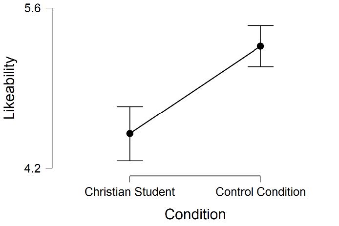
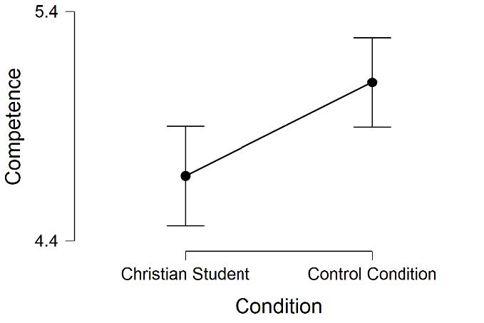
If we look at the Descriptives Plot in our JASP output, we can see a graphical representation of our results. This graph plots the means for each of our groups on the dependent variable. Looking at the y-axis, you can see the label for our dependent variables “likeability” and “competence.” Looking at the x-axis, you can see the label for the levels of our independent variable “Christian Student” and “Control Condition.” Just looking at the means represented on this plot, it is easy to see that the Control Condition was rated as more likeable and competent than the Christian Student condition.
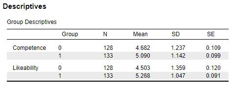
If we look at our Group Descriptives table, we can see the sample sizes (N), means (Mean), standard deviations (SD), and standard errors (SE) for both groups. We will want to include this information in our results. Formatting this information into APA format, we might report:
There were 128 faculty randomly assigned to the Christian Student condition and 133 faculty randomly assigned to the Control Condition who participated in this study. Faculty in the Control Condition rated the applicant as having a higher level of likeability (M = 5.27, SD = 1.05), compared to faculty ratings in the Christian Student Condition (M = 4.50, SD = 1.36). Additionally, faculty in the Control Condition rated the applicant as having a higher level of competence (M = 5.09, SD = 1.14), compared to faculty ratings in the Christian Student Condition (M= 4.68, SD= 1.24).
Interpreting the Practical Significance of Independent Samples t Tests
Now that we have interpreted the statistical significance, we will look at the practical significance by looking at our effect size. A significant p value tells us that there is a difference in mean level of our dependent variables (likeability and competence) between the Christian Student and Control Conditions in this study, but the effect size tells us how big this difference is. Unlike p values, the Cohen’s d effect size test is not impacted by the sample size.
Reminder: Cohen’s d Effect Sizes
| Effect Size | Strength |
| .2 | Small |
| .5 | Medium |
| .8 | Large |
We obtained Cohen’s d values of -.63 for Likeability and -.34 for Competence. We obtained a small effect size for faculty Competence ratings and a medium effect size for faculty ratings of applicant Likeability.
Reporting in APA Format
What do you need to report in your results?
| Value (Notation) | Levene’s Statistic |
| Means (M) | Standard Deviations (SD) |
| Test Statistic (t) | Degrees of Freedom (df) |
| Probability (p) | Effect Size |
| Cohen’s d | Confidence Interval |
| Skewness and Kurtosis | Boxplot |
Bonferroni Correction
For this example, we had three separate hypotheses, one for each of our dependent variables. Because we are conducting multiple comparisons with the same sample, we need to correct for experimentwise or familywise error to keep our Type I error rate at 5%. With an alpha level of .05, we have a 5% chance of making a Type I error (rejecting a null hypothesis that is true).
| Hypothesis One | Comparing the mean faculty rating of applicant likeability for the Christian Student Condition with the Control Student Condition. | 5% Type I Error Rate |
| Hypothesis Two | Comparing the mean faculty rating of applicant competence for the Christian Student Condition with the Control Student Condition. | 5% Type I Error Rate |
| 10% Total Type I Error Rate |
To reduce our chance of making a Type I error with multiple comparisons, we can conduct a Bonferroni Correction. To do this, we divide our alpha level (ɑ) by the number of comparisons (k). In this example, our alpha level is .05 and we had a total of three comparisons.
PCritical = ɑ ÷ k
PCritical =.05 ÷ 2 = 0.025
Given the p critical results above, we would need to interpret our p values with an adjusted alpha level or Bonferroni Correction, of 0.025. This means, in order to reject our null hypotheses, all of our p values would need to be below 0.025 in order to be considered statistically significant. Prior to reporting your analyses, you would add to report:
Analyses were conducted with a Bonferroni adjustment of p < .025.
Putting it All Together
Now, let’s write up the results of our test combining everything we’ve done so far, including the test of assumptions, and the results of the t test.
A set of independent samples t test were conducted to determine if there were mean differences in faculty ratings of a PhD applicant’s likeability and competence between faculty assigned to read application materials for a Christian Student versus a Control Student condition. There was one outlier for likeability for the Control Condition and six outliers for the competence for the Christian Student condition, as assessed by the inspection of a boxplot. Likeability and competence were normally distributed, with skewness and kurtosis values between -2 and +2. There was homogeneity of variances, as assessed by the Levene’s test for competence (p > .05), but not for likeability (p < .05).
Analyses were conducted with a Bonferroni adjustment of p < .025. Faculty in the Control condition rated PhD applicants as having higher levels of likeability and competence. Specifically, faculty in the Control Condition rated the applicant as having a higher level of likeability (M = 5.27, SD = 1.05), compared to faculty ratings in the Christian Student Condition (M = 4.50, SD = 1.36), t (238.68) = -5.09, p < .001, d = -.63. Additionally, faculty in the Control Condition rated the applicant as having a higher level of competence (M = 5.09, SD = 1.14), compared to faculty ratings in the Christian Student Condition (M= 4.68, SD= 1.24), t (259) = -2.77, p < .01, d = -.34.
Real World Meaning
When we interpret the real world meaning of a study, we want to take out any statistical jargon and describe the results of the study in a way that is easy to understand by people who do not know anything about statistics. How would you describe the results to your roommate, sibling, parent, or neighbor? For this study, we want to not only say there are differences between faculty ratings when reading mock application materials for a Christian Student compared to a Control Student where their religiosity is not mentioned, but we want to describe which group has higher or lower scores. We also need to translate our outcome variables “likeability and competence” into terms that are easy to understand by others. Thankfully the names of these variables are fairly straightforward, but that is not always the case in psychological research. For example, if I was telling my brother the real world meaning of our results, I would say:
Researchers found that biology faculty members that read application materials for a fake potential PhD student where their religion was not discussed perceived the applicant as more likeable and more competent than biology faculty that read fake application materials for a Christian Student who discussed their religion and evangelical religious activities. The results of this study suggest that individuals within the science community may be more likely to perceive PhD Christian students as less likeable and less competent than PhD students who did not explicitly state their religious beliefs.
Barnes, Truong, and colleagues (2020) conducted additional analyses that showed that atheist faculty showed a stronger bias against the Christian Student condition compared to faculty who identified as Christian themselves. The authors suggested this may be due to a historical bias against science in fundamentalist and evangelical Christian beliefs (Marsden, 2015; Numbers, 2006). This includes, for example, movements by these groups to teach “creationism in US science classes in an attempt to discredit evolution to students” (Barnes et al., 2020, p. 12; Berkman & Plutzer, 2011). However, the scenario faculty read in this study did not include any mention of the fake graduate student applicant’s political beliefs and may have used stereotypes to judge the candidate. The authors conducted a total of three separate studies. We will analyze data from their second study in a future assignment to see if they observed similar results when comparing graduate student applications that mentioned activities that were either Christian, Atheist, or a Control condition.
References
Barnes, M. E., Truong, J. M., Grunspan, D. Z., & Brownell, S. E. (2020). Are scientists biased against Christians? Exploring real and perceived bias against Christians in academic biology. PLoS ONE, 15(1). https://doi.org/10.1371/journal.pone.0226826
Berkman, M. B. & Plutzer, E. (2011). Defeating creationism in the courtroom, but not in the classroom. Science, 331, 404-405.
Ecklund, E. H., Johnson, D. R., Scheitle, C. P., Matthews, K. R. W., & Lewis, S. W. (2016). Religion among Scientists in International Context: A New Study of Scientists in Eight Regions. Socius : Sociological Research for a Dynamic World, 2, 237802311666435–. https://doi.org/10.1177/2378023116664353
Marsden, G.M. (2015). Religious discrimination in academia. Society, 52(1), 19-22.
Numbers, R. L. (2006). The Creationists: From scientific creationism to intelligent design. Harvard University Press.
Pew Research Center (2019). In U.S., decline of Christianity continues at rapid pace. Retrieved from https://www.pewforum.org/2019/10/17/in-u-s-decline-of-christianity-continues-at-rapid-pace/
Authors
This guide was written and created by Kelsey L. Humphrey, Ruth V. Walker, PhD, and Erin N. Prince.
Acknowledgements
We would like to thank M. Elizabeth Barnes, Jasmine M. Truong, Daniel Z. Grunspan, and Sara E. Brownell for making their data available through PLoS One. Additionally, we appreciate Dr. Kristen Black’s edits and suggestions during the creation of this guide.
Copyright
CC BY-NC-ND: This license allows reusers to copy and distribute the material in any medium or format in unadapted form only, for noncommercial purposes only, and only so long as attribution is given to the creator.