
5 Running and Interpreting a Chi-Square Test in JASP
Ashlyn A. Moraine; Dr. Hannah J. Osborn; and Ruth Walker
Download Data Sets:
The terms used to describe their ethnic identity by people who can trace their origins back to South America, Latin America, and Spain varies between individuals and have changed over time. In a national survey of 5,103 Hispanic adults in 2013, the Pew Research Center found that the majority of participants defined their ethnic identity in terms of their specific Hispanic origin, particularly those who immigrated to the U.S. from other countries. For example, using terms that indicated a geographical origin such as Dominican, Cuban, South American, Puerto Rican, or Salvadoran. The rest of the participants used the terms Hispanic, Latino, or American, with higher proportions of native-born participants using these terms – particularly amongst third generation members of the Hispanic community. Recently, a gender-neutral term, Latinx, has been gaining momentum as a new way of describing the Hispanic population in the U.S. Why use the term Latinx instead of Latino, Latina, or Hispanic? As one younger participant in a national survey explained, “Latinx is a more inclusive term to use for those who do not choose to identify with a certain gender. The terms Latino and Latina are very limiting for certain people” (Noe-Bustamante, Mora, & Hugo Lopez, 2020).
Although Google trend data between 2011-2020 shows a rise in the prevalence of Latinx, the terms Latina, Latino, and Hispanic continue to be more widely used.
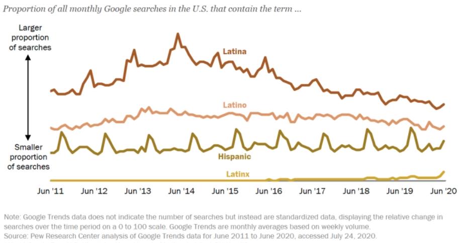
Pew Research Center Graph (2020)
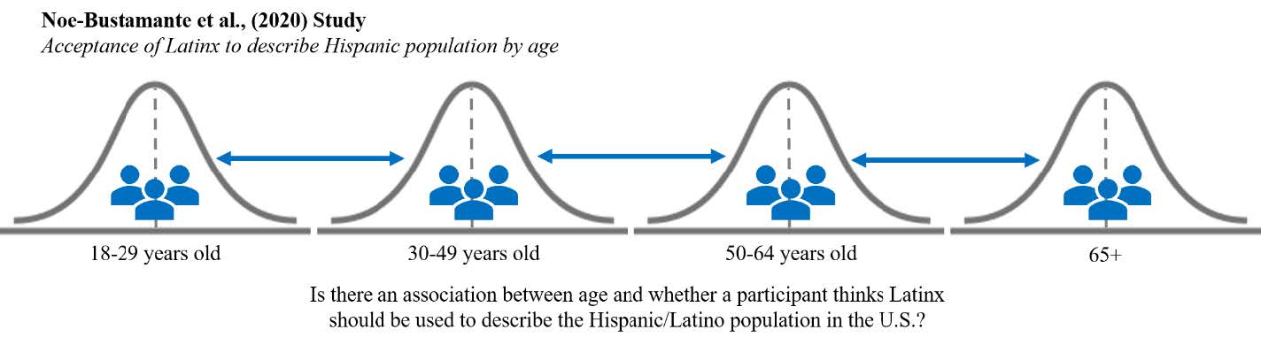
A recent survey by researchers at the Pew Research Center found that 76% of U.S. Hispanic/Latino adults surveyed in late 2019 had not heard of the term Latinx (Noe-Bustamante et al., 2020); however, of the 23% who had heard of the term, only 3% reported using it to describe themselves. Additionally, younger participants between 18-29 years old were the most likely to have heard of the term Latinx, with 42% saying they were familiar with the term compared to only 7% of older adults 65 years and older. When asked if they thought Latinx should be adopted as a pan-ethic term for U.S. Hispanics, the majority of participants (61%) said they prefer the term Hispanic, 29% preferred Latino, and only 4% said they preferred Latinx. Knowing there are age differences in terms of how aware participants are of the term Latinx, are there also age differences in whether participants think the term Latinx should be adopted by the Hispanic/Latino population? Let’s find out!
For this walk-through example, we are going to focus on two of these variables: “Age” and “Latinx.” We want to see whether there is an association between age groups (18-29, 30-49, 50-64, and 65+) and whether a person thinks Latinx should be used to describe the Hispanic or Latino population (Yes, No). To answer this question, we will conduct a chi-square test.
Hypotheses
Let’s review our hypotheses for this example we are about to run in JASP.
The null hypothesis is:
Conceptual H0: There is no significant association between age groups and whether a person thinks Latinx should be used to describe the Hispanic or Latino population
Mathematical H0: The observed frequencies are equal to the expected frequencies.
The alternative hypothesis is:
Conceptual H1: There is a significant association between age groups and whether a person thinks Latinx should be used to describe the Hispanic or Latino population
Mathematical H1: The observed frequencies are not equal to the expected frequencies.
JASP Analyses
In order to run analyses, the first thing we need to do is open the data set we will be working with. To do this, open JASP and follow the steps below:
File → Open → Computer → Browse → Select the ‘Chi Square Class Practice Data (Pew Research Center, 2020)’ csv file wherever it is saved on your computer.
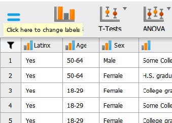
Once the data is open in JASP, we will need for first change the data labels for our variables so that we know what the values mean when we run analyses. There are multiple variables in the dataset, however, we are going to focus on Latinx and Age for this example. See the following bulleted list for a description of how each variable was coded.
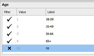
- Latinx: 1 = ‘Yes’, 2 = ‘No’
- Age: 1 = ’18-29, 2 = ’30-49’, 3 = ’50-64’, 4 = ‘65+’, 99 = ‘Refused’
- Sex: 1 = ‘Male’, 2 = ‘Female’, 99 = ‘Refused’
- Education: 1 = ‘College graduate’, 2 = ‘Some college’, 3 = ‘H.S. graduate or less’, 99 = ‘Refused’
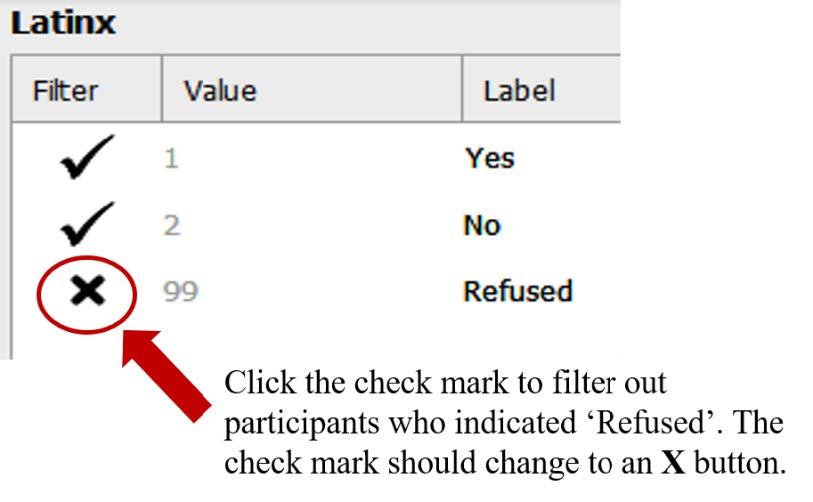
Before we do anything else, let’s get our dataset to reflect the participants we want to analyze in this chi-square test. Remember, we are comparing participants in different age groups and whether they believe the term Latinx should be used to describe the Hispanic or Latino population. To do this, we want to first make sure we filter out any participants who did not respond to either prompt. For both Latinx and Age we are going to filter out participants with the “Refused” label.
To change the numerical data into our categorical labels, you will take your cursor and hover over the column for the variable you want to change. Let’s do ‘Latinx’ together, and then you can do the others on your own. Hover over the variable column ‘Latinx’. When you see a pop up saying, “click here to change labels” click on it. To change the labels, click on the 1 under the Label column and type ‘Yes’ and hit enter. Then click on the 2 under the Label column and type ‘No’ and hit enter. This will change your labels for the variable ‘Latinx’.
To filter out participants, we will click the check mark next to the responses we want filtered out. In the variable labels box, click the check mark next to the ‘99’ label, and it will turn the button into an X button.
Repeat the above steps to filter out participants who refused to provide their age for our “Age” variable.
Assumption Testing
There are just three statistical assumptions for a chi-square test. The first two deal more with the research design, and the third assumption we will test when we actually run the chi-square test.
Assumption 1: Two Categorical Variables.
Yes. In this example, we have two categorical, nominal variables. Our first variable, ‘Latinx’ is a dichotomous categorical variable, where participants responded that they either think this term should be used to describe the Hispanic or Latino population, or not. Our second variable, ‘Age group’, is also a categorical variable, because participants either indicate their age as ’18-29’ or ’30-49’ or ’50-64’ or ‘65+.’ Because both of our variables are categorical variables, we meet this assumption.
Assumption 2: Independence of Observations.
Yes. We can assume that we have independence of observations because each participant represents a unique combination of the different levels of each variable. That means that for any given participant, they are only in one of the total possible “cells” in the contingency table. For instance, a participant is in one of eight possible cells in the following contingency table. Because participants can only be in one of these cells based on their specific categories, we can assume independence of observations. So, we have met this assumption.
| 18-29 years old | 30-49 years old | 50-64 years old | 65+ | |
| Yes Latinx should be used to describe the Hispanic/Latino population. |
18-29-year olds who said “Yes” | 30-49-year olds who said “Yes” | 50-64-year olds who said “Yes” | 65+ year olds who said “Yes” |
| No Latinx should NOT be used to describe the Hispanic/Latino population. |
18-29-year olds who said “No” | 30-49-year olds who said “No” | 50-64-year olds who said “No” | 65+ year olds who said “No” |
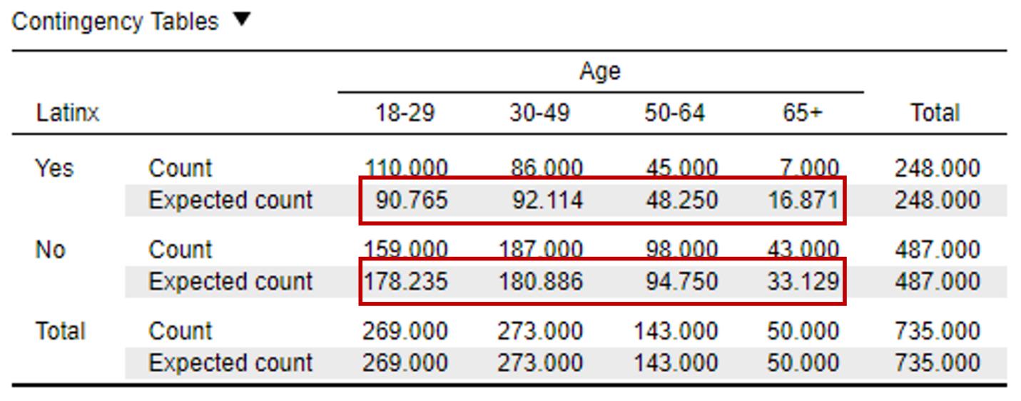
Assumption 3: Expected Counts Greater than Five.
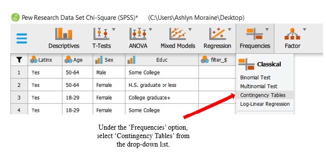
To determine whether our expected counts are greater than five, we need to have JASP run the chi-square test. To run the chi-square test, go to ‘Frequencies’ at the top of the JASP window and select ‘Contingency Tables’, as shown in the following image.
Primary Analyses
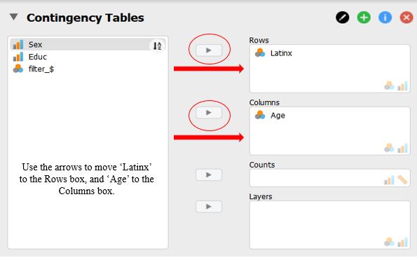
Now we need to choose which variables to move into the ‘Row’ and ‘Column’ boxes. Ultimately, it does not matter how you choose to organize your table, so choose the format that will work the best for you. For this dataset we will use the top arrow to move the variable ‘Latinx’ into the ‘Row’ box. Click the other arrow to move the ‘Age’ variable to the ‘Column’ box.
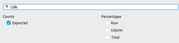
To test our third assumption (expected counts greater than five), click on the ‘Cells’ and select the “Expected” check mark under the “Counts” heading.
In the output window, take a look at the table labeled “Contingency Table”. The rows that are labeled “Count” refer to the observed counts based on participants responses. Take a look at the expected counts highlighted in the image below with red boxes. What we can see for each of our cells is that our expected counts are greater than five for each cell. This means that we have satisfied assumption three and can move on with the chi-square test!
| Can You Read the Contingency Table?
Let’s make sure you can read the contingency table below. How many people in our sample are middle-aged (50-64 years old) and think Latinx should be used to describe the Hispanic/Latino population in the United States? To figure this out, we need to make sure we’re looking at the right cell. We’ll want to look at the row labeled “Yes”, and within this row, pay attention to the row labeled ‘Count’. Now that we’re in the right row, we need to make sure we’re in the right column. We want people who are 50-64 years old. If we look for the cell based on that combination of categories, you should end up at a value of 45. This means that 45 50-64-year olds indicated they thought Latinx should be used to describe the Hispanic/Latino population in the U.S. |
To report this assumption test in APA format, you could say:
A chi-square test for association was conducted between age group and whether people think the term Latinx should be used to describe the Hispanic or Latino population. All expected cell frequencies were greater than five.
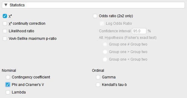
To run the chi-square test and select all other pieces of information we’ll need, click on the ‘Statistics’ option in the test menu. You’ll see that the chi-square test is already selected. All we’ll need to add now is Phi and Cramer’s V to get the effect size. To do this, select the checkbox labeled “Phi and Cramer’s V.”
Interpreting and Reporting the Statistical Significance of the Chi-Square Test
To determine whether the chi-square test is statistically significant, let’s look at the following chi-square test output.
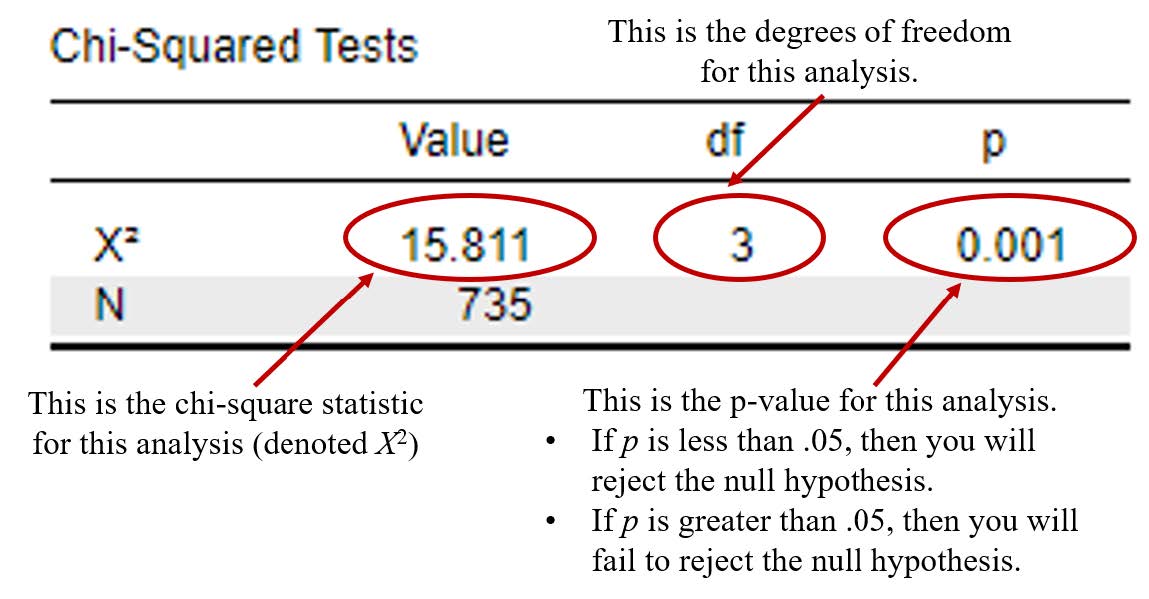
To interpret the statistical significance of the chi-square test, we want to look at the p value. If the p value is less that our alpha level of .05, we will reject the null hypothesis (indicating that there is a significant association between age groups and whether a person thinks Latinx should be used to describe the Hispanic or Latino population). If the p value is greater than our alpha level of .05, then we will fail to reject the null hypothesis (indicating there is not a significant association between our variables).
In this example, you can see from the “Chi-Squared” table that our p value is < .001, which is less than the alpha of .05. Therefore, we will reject our null hypothesis – indicating that there is a significant association between age groups and whether a person thinks Latinx should be used to describe the Hispanic or Latino population.
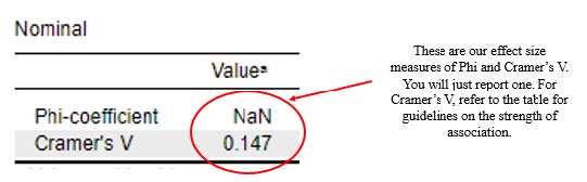
Next we will look at the “Nominal” table to report our effect size. Phi is only available when you have a 2×2 contingency table. Because we have a 2×4 contingency table, we will report the Cramer’s V value depicted in the following table.
Writing the results of the chi-square test in APA format follows this general format:
X2(df) = chi-square statistic, p < .05 or p > .05, ɸ = Phi coefficient OR Cramer’s V = Cramer’s V value
So, plugging in our results into this format should look like this:
X2(3) = 15.81, p < .05, Cramer’s V = .15
Interpreting the Practical Significance of the Chi-Square Test
Now that we have interpreted the statistical significance of the chi-square test, let’s consider the practical significance of this test. Remember, a significant p value tells us that there is a significant age groups and whether a person thinks Latinx should be used to describe the Hispanic or Latino population. The effect size, then, tells us how meaningful or strong this association is. That is, the effect size tells us how strongly related our two variables are to one another.
For the purposes of this analysis, because we are interpreting a 2 x 4 crosstabulation, we will interpret Cramer’s V. Let’s refer back to the Cramer’s V guidelines for strength of association for our degrees of freedom = 3. A small effect is .06, a medium effect is .17, and a large effect is .29. We obtained a value of .15 (almost a medium effect), so we would say that the strength of association age groups and whether a person thinks Latinx should be used to describe the Hispanic or Latino population is small to medium.
Guidelines for Interpreting Cramer’s V
| Small Effect Size | Medium Effect Size | Large Effect Size | |
| dfRC = 1 | .10 | .30 | .50 |
| dfRC = 2 | .07 | .21 | .35 |
| dfRC = 3 | .06 | .17 | .29 |
| dfRC = 4 | .05 | .15 | .25 |
| dfRC = 5 | .05 | .13 | .22 |
In addition to reporting Phi and Cramer’s V effect size statistics as a measure of practical significance, odds ratios are also common when making a 2×2 comparison (e.g., you have two dichotomous variables). Because odds ratios can only be calculated for 2×2 contingency tables, we are unable to use that method to gain additional understanding from our current data since we are working with a 2×4 design with four levels of our age variable. However, we could potentially run planned comparisons. Planned comparisons are comparisons that need to be chosen a priori or before we run our test as part our initial study hypotheses. For example, given the data shared in the Pew Research Report about awareness of the Latinx term being higher in younger adults, we might plan to compare the 18-29 year group to the 30-49 year old group, the 50-64 year old group, and the 65+ year old group to see if there is a significant association when broken down and compared individually. To do this, we would have to go back to our “Age” variable and filter out the groups we are not currently comparing.
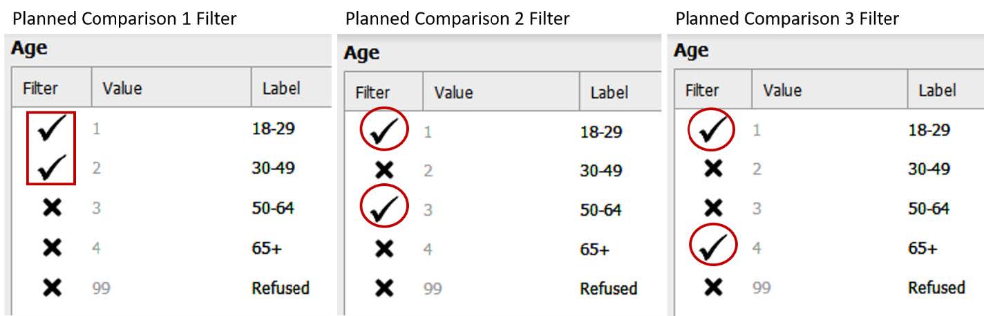
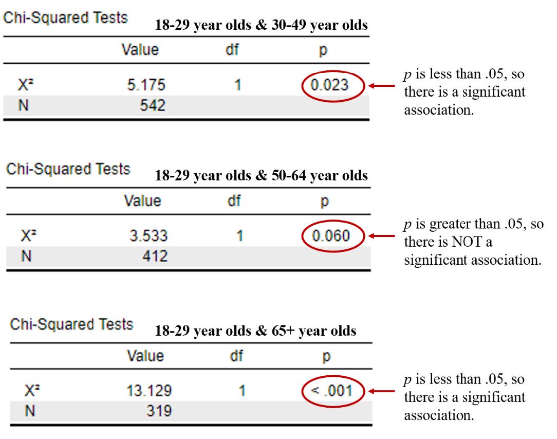
We will then look at our Chi-Square results for each of the planned comparisons, illustrated in the following images. The first image includes the Chi-Square test results for our first comparison (18-29-year-old group compared to the 30-49-year-old group). Then we seeour second comparison (18-29-year-old group compared to the 50-64-year-old group), and our third comparison (18-29-year-old group compared to the 65+ year old group). Remember, we want a p value that is less than .05 in order to conclude there is a significant association. Our probability value is significant, or less than .05, for the first and the third comparison but not for the second.
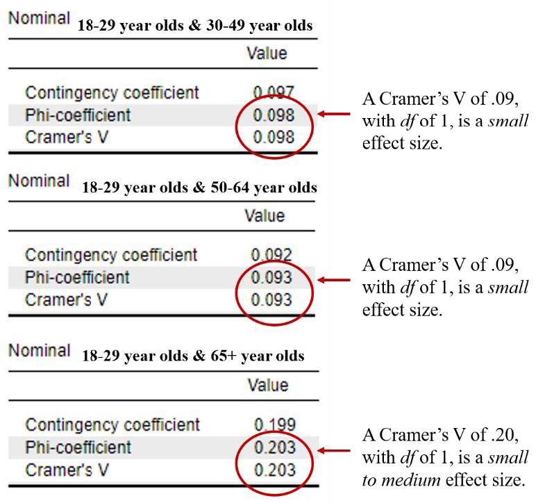
We will now look at our effect size results for each of the planned comparisons, illustrated in the following images. The first image includes the effect size results for our first comparison (18-29-year-old group compared to the 30-49-year-old group), our second comparison (18-29-year-old group compared to the 50-64-year-old group), and our third comparison (18-29-year-old group compared to the 65+ year old group). The first two comparisons have small effect sizes, and the third comparison between the 18-29-year-old group and 65+ year old group is small to medium.
Looking back at our original contingency table, we would be able to conclude that the young adult group (18-29-year olds) are significantly more likely to believe that Latinx should be used to describe the Hispanic/Latino population in the United States compared to 30-49 year olds and older adults 65 years and older; however, this difference in preferences is relatively small.
Reporting in APA Format
What do you need to report in your results?
| Value (Notation) | |
| Chi-Square Test | Chi-Square Value (X2) |
| Degrees of Freedom (df) | Probability (p) |
| Effect Size | Phi (ɸ) or Cramer’s V |
| Odds Ratio | Assumptions |
| Expected Counts > 5 |
Putting it All Together
Participants were current American Trends Panel (ATP) panel members who identified as being Hispanic. A chi-square test was conducted to examine whether there was an association between age groups and whether a person thinks Latinx should be used to describe the Hispanic or Latino population All expected cell frequencies were greater than five. There was a statistically significant association between
age groups and whether a person thinks Latinx should be used to describe the Hispanic or Latino population, X2(3) = 15.81, p < .05, Cramer’s V = .15. This was a small to medium association. Planned comparisons were completed to compare the 18-29-year-old age group with the 30-49-year-old group, the 50-64-year-old group, and the 65+ year old group. There was a significant association between age group and whether a person thinks Latinx should be used to describe the Hispanic or Latino population for the first planned comparison (18-29-year-old group and 30-49-year-old group), X2(1) = 5.18, p < .05, Cramer’s V = .09, a small association. There was also a significant association between age group and whether a person thinks Latinx should be used to describe the Hispanic or Latino population for the third planned comparison (18-29-year-old group and 65+ year old group), X2(1) = 13.13, p < .001, Cramer’s V = .20, a small to medium association. However, there was not a significant association between age group and whether a person thinks Latinx should be used to describe the Hispanic or Latino population for the second planned comparison (18-29-year-old group and 50-64-year-old group), X2(1) = 3.53, p > .05, Cramer’s V = .09.
Real-World Meaning
Remember, when we’re explaining the results of statistical analyses in real-world terms, we want to try our best to explain this to someone who has never taken statistics. We want them to be able to understand the results of the analyses without knowing how to do them. An effective way to do this is to briefly put the statistical test in the context of the research question, explain what the researchers did, and then describe what they found. It can also be helpful to put the results of the analyses back into the context of the original research question and attempt to answer a “so what?” question. If I was telling my friends about the results of these analyses, I would tell them that different age groups feel differently about using the term Latinx to describe the Hispanic/Latino population in the United States. Recent data suggests younger adults are more likely to believe Latinx term should be used compared to older generations.
References
Hugo Lopez, M. (2013). Hispanic Identity. Pew Research Center. Retrieved from https://www.pewresearch.org/hispanic/2013/10/22/3-hispanic-identity/
Noe-Bustamante, L., Mora, L., & Hugo Lopez, M. (2020). About one-in-four U.S. Hispanics have heard of Latinx, but just 3% use it. Pew Research Center. Retrieved from https://www.pewresearch.org/hispanic/2020/08/11/about-one-in-four-u-s-hispanics-have-heard-of-latinx-but-just-3-use-it/
Authors
This guide was written and created by Ashlyn A. Moraine, Ruth V. Walker, PhD, and Hannah J. Osborn, PhD.
Acknowledgements
We would like to thank the Pew Research Center for generously making their data available for secondary analysis. Additionally, we appreciate Dr. Kristen Black’s edits and suggestions during the creation of this guide.
Copyright
CC BY-NC-ND: This license allows reusers to copy and distribute the material in any medium or format in unadapted form only, for noncommercial purposes only, and only so long as attribution is given to the creator.