
3 Running and Interpreting a One-Way ANOVA in JSAP
Ashlyn A. Moraine; Dr. Hannah J. Osborn; Erin N. Prince; and Ruth Walker
Download Data Sets:
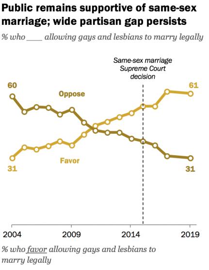
Minority stress theory describes how experiences with stigma, prejudice, and discrimination connect to the physical and mental health of sexual minority people (Meyer, 2003). As societal attitudes toward sexual minorities (e.g., gay, lesbian, and bisexual people) continues to improve, this theory would suggest that physical and mental health outcomes for this population should also improve. As you can see from the following Pew Research Center (2019) graph, attitudes in favor of same-sex marriage, for example, have increased significantly since 2004. Additionally, the US Supreme Court banned employment discrimination based on gender identity or sexual orientation in 2020. Using minority stress theory, these improvements in social context (e.g., attitudes, legislation) would suggest that sexual minorities have improved physical and mental outcomes. Meyer and colleagues (2021) conducted a study to see if there is support for this. Specifically, they wanted to know if minority stress is reduced in younger generations of sexual minorities, compared to older generations of sexual minorities. They did this by comparing the outcomes of three different cohorts of sexual minorities: Equality Cohort, aged 18-25 years (n = 670), Visibility Cohort, aged 34-41 years (n = 372), and Pride Cohort, aged 52-59 years (n = 476).
Meyer and colleagues (2021) examined numerous variables, both categorical and continuous. For the purposes of this guide, we will be using these two continuous variables as our dependent variables: Connection with the LGBT community and life satisfaction. We will need to run two One-way ANOVA’s to see if either dependent variable has statistically significant differences between group means for our independent variable or factor (cohort).
Connection with the LGBT community
This variable measures the desire and/or strength of a participant’s connection to the LGBT community. Scores can range from 1-4 and are based on a 4-point Likert scale (“agree strongly” to “disagree strongly”). Lower scores represent lower connection with the LGBT community.
Life satisfaction
This variable measures the degree to which participants are satisfied with their life. This variable is measured by asking participants to rate 5-items on a7-point Likert scale (“disagree strongly” to “agree strongly”). Lower scores represent lower life satisfaction.
Hypotheses
We have two different dependent variables we are looking at in this example: (1) Connection with the LGBT Community and (2) Life satisfaction. This means that we will have two different sets of hypotheses.
The null hypotheses are:
- Connection with the LGBT Community
- Conceptual H0: There are no significant group mean differences on connection with the LGBT community between the younger, middle-aged, and older adult groups.
- Mathematical H0: There are no significant differences between the population means for the younger, middle-aged, and older adult groups on connection with the LGBT community; Myounger = Mmiddle= Molder
- Life satisfaction
- Conceptual H0: There are no significant group mean differences on life satisfaction between the younger, middle-aged, and older adult groups.
- Mathematical H0: There are no significant differences between the population means for the younger, middle-aged, and older adult groups on life satisfaction; Myounger = Mmiddle= Molder.
The alternative hypotheses are:
- Connection with the LGBT Community
- Conceptual H2: There is at least one significant group mean difference on connection with the LGBT community between the younger, middle-aged, and older adult groups.
- Mathematical H2: There is at least one significant difference between the population means for the younger, middle-aged, and older adult groups on connection with the LGBT community; Myounger ≠ Mmiddle ≠ Molder.
- Life satisfaction
- Conceptual H1: There is at least one significant group mean difference on life satisfaction between the younger, middle-aged, and older adult groups.
- Mathematical H1: There is at least one significant difference between the population means for the younger, middle-aged, and older adult groups on life satisfaction; Myounger ≠ Mmiddle ≠ Molder.
JASP Analyses
In order to run analyses, the first thing we need to do is open the data set we will be working with. To do this, open JASP and follow the steps below:
File → Open → Computer → Browse → Select the “One-Way ANOVA Practice Data Set (Meyer et al. 2021)” JASP file wherever it is saved on your computer.
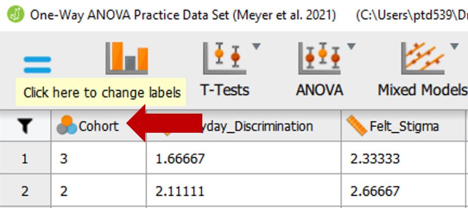
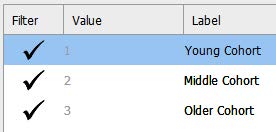
Once the data set is open in JASP, we will change the data labels for our condition variable so that we can see which groups are being compared when we run the omnibus and post hoc tests. Currently the condition column has either a 1, 2, or 3 for each participant. Based on Meyer et al.’s (2021) codebook, we will need to change these labels so that 1 = ‘young cohort’, 2 = ‘middle cohort’, 3 = ‘older cohort.’ To change the numerical data into our categorical labels, you will take your cursor and hover over the ‘Condition’ column. When you see a pop up saying, “click here to change labels” click on it. To change the labels, click on the 1 under the Label column and type ‘younger.’ Then click on the 2 under the Label column and type ‘middle, and so-on until all conditions are appropriately labeled. After you have changed the labels, you can close the window by clicking on the X button.
Assumption Testing
There are six statistical assumptions that data must meet in order to run a one-way ANOVA. Many of these assumptions will look familiar, as they are quite similar to those required to run an independent measures t test – we’re just adding more groups! Assumptions 1 through 3 have to do more with the research design, and assumptions 4 through and 6 refer to those which data must meet in order to run the statistical test. Let’s consider whether our data meet these assumptions:
Assumption 1: Categorical Independent Variable.
Yes. We have one independent variable (experimental condition), and participants have been assigned to one of three levels of that independent variable based on their age. Therefore, participants are in one ‘category’ of the independent variable, so we meet this assumption.
Assumption 2: Continuous Dependent Variable.
Yes. We have dependent variable(s) (‘life satisfaction’ and ‘community connectedness’) and these dependent variables are single items based on self-reports measured on Likert-type scales. In psychological research, Likert-type responses are treated as continuous data. Therefore, we meet this assumption.
Assumption 3: Independence of Observations.
Yes. Our participants were assigned to one of the three possible levels of the independent variable, and because no participant can be in more than one age group, we can assume that there is no relationship between the observations in each group. This assumption has been met.
Assumption 4: Normal Distribution.
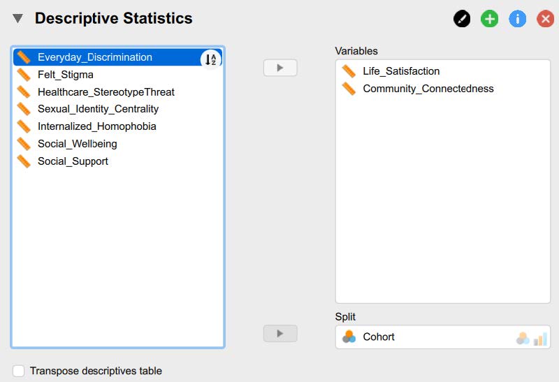
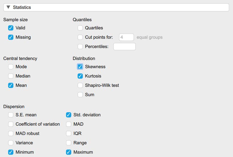
To check our data for Assumptions 4 and 5, we will need to utilize the Descriptives tab. When the “Descriptive Statistics” window opens, move the dependent variables (‘life satisfaction’ and ‘community connectedness) to the “Variables” box. Then, move our factor or independent variable (‘Cohort’) to the “Split” box so that we get plots for each group.
Under the “Plots” tab, select:
- “Customizable Boxplots”: “Boxplots,” “Boxplot element” and “Label outliers”

Under the “Statistics” tab, select:
- Under “Central Tendency,” select “Mean”
- Under “Distribution,” select “Skewness” and “Kurtosis”
- Under “Dispersion,” select “Minimum,” “Maximum,” and “Std. deviation”
Although there are multiple ways to determine if the dependent variable is normally distributed for each group of our independent variable, for this course we will focus on interpreting the skewness and kurtosis statistics. We want skewness and kurtosis values at are between -2 and +2. Looking at the values on the following output copied, we can see our skewness and kurtosis values for the dependent variable for all of our groups are within the acceptable range of -2 and +2 across both of our dependent variables.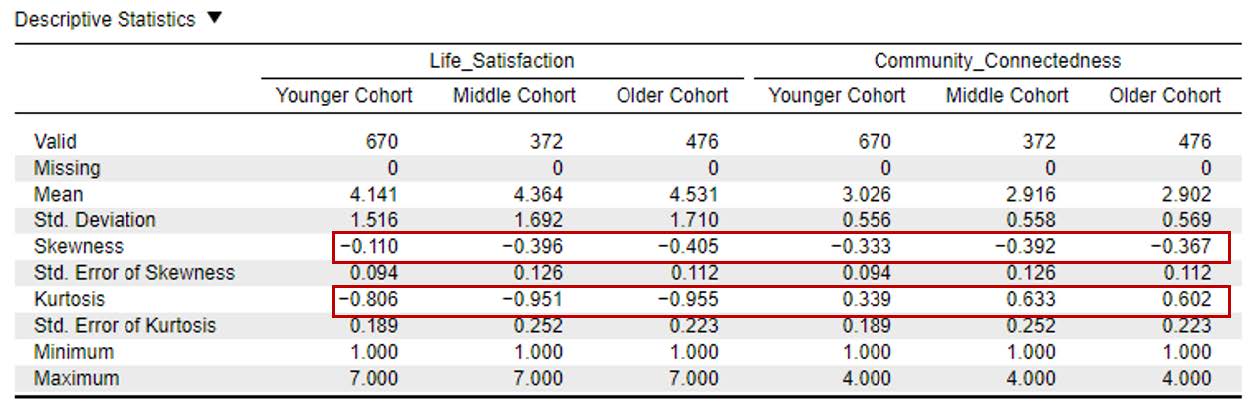
To report these results in APA format, we can write:
The scores on both life satisfaction and community connectedness were normally distributed across all conditions, as skewness and kurtosis statistics fell within the acceptable range of -2 and +2.
Assumption 5: No Outliers.
To determine if we have any outliers, we will look at the boxplots in our JASP output. If we have any outliers, they would be outside the top and bottom lines or whiskers. As you can see from the boxplots, we do have outliers in our data, and we have violated this assumption. Which means we have to decide whether we want to keep the outliers, transform the outliers, or remove them. Given that outliers are especially common in datasets with large samples (as ours is; N = 1,458), and that we have so many, we will keep these outliers in our dataset in order to avoid removing a significant amount of datapoints from our model (something that is generally discouraged, Faraway, 2015). Instead, we will model how to run the analyses as normal with outliers present, and at the end of this guide, will run the analyses with those outliers removed to examine whether the results remained the same.
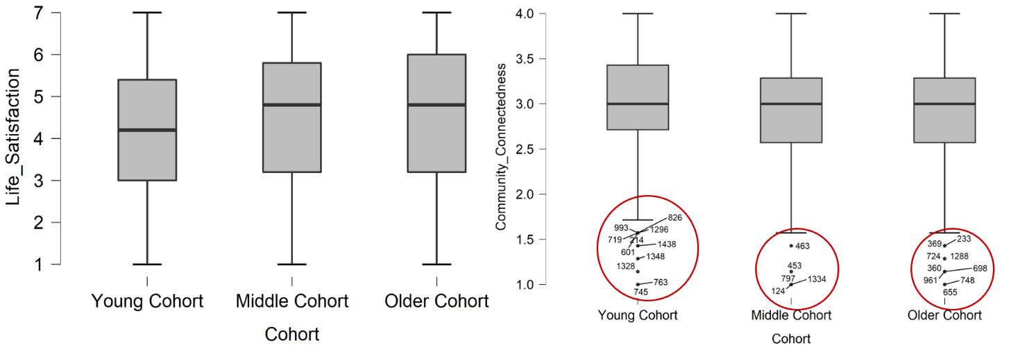
To report this using APA format, we would write:
There were no outliers identified on the life satisfaction scores; however, there were several outliers across all three cohorts for the community connectedness variable, as assessed by the inspection of a boxplot. We decided to retain these outliers given the large sample size to avoid removing a large number of datapoints from the model.
Assumption 6: Homogeneity of Variance.
Checking for the homogeneity of variances assumption is part of the overall one-way ANOVA test. Let’s move onto our primary analyses, and complete checking this assumption in that section.
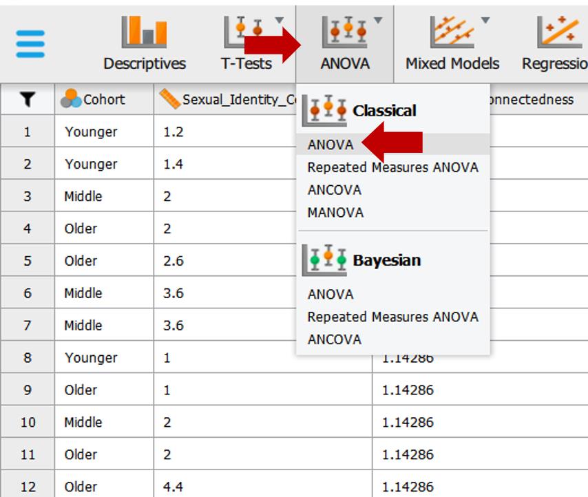
Primary Analyses: Omnibus Test for Community Connectedness.
To run a one-way between subjects ANOVA, we will begin by testing the omnibus effect, and then follow up with a section on Post hoc analyses. To run the one-way ANOVA, go to ANOVA at the top of the JASP screen and select ‘ANOVA’. See the image below:
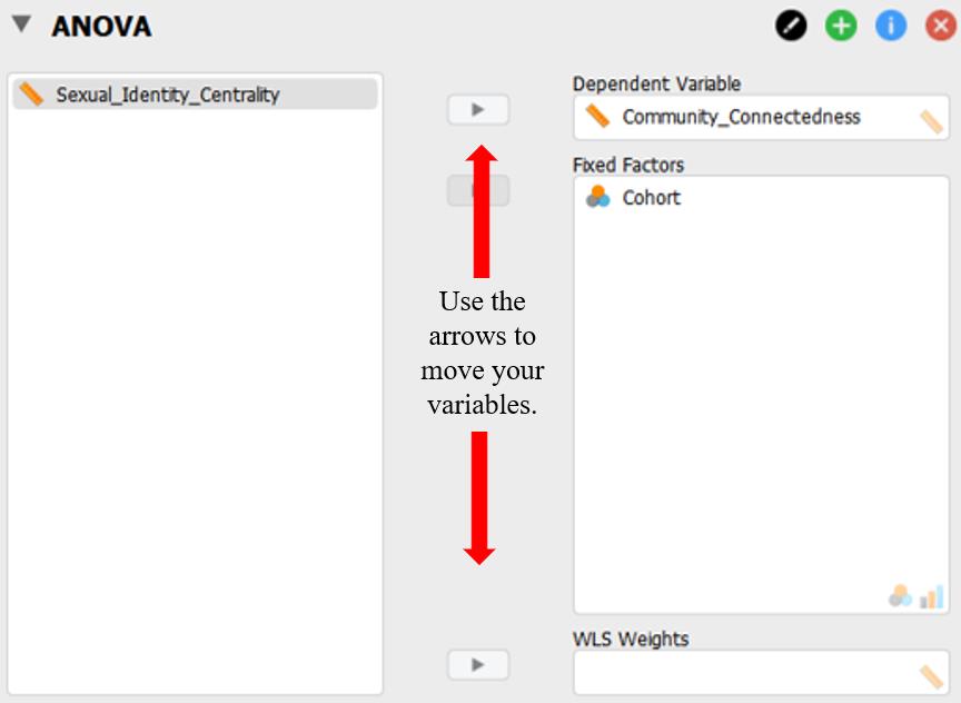
First, we need to move our dependent variable [community connectedness] to the “Variables” box and our independent variable [cohort] to the “Fixed Factors” box.
- We are then going to ask JASP to run the various analyses we will need to interpret for our test by clicking on the appropriate boxes in the window.
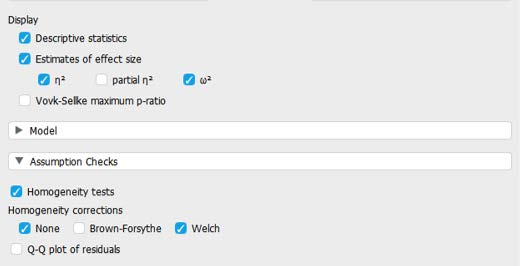
- Under “Display” we will want to check ‘Descriptive statistics’ and ‘Estimates of effect size’ – ‘eta- squared’ and ‘omega-squared’
- Under “Assumption Checks” select ‘Homogeneity tests’; under “Assumption corrections” select ‘None’ and ‘Welch’
Now that we have asked JASP to run the appropriate analyses for the omnibus test, let’s first look to see if we’ve met the assumption for homogeneity of variances. In your output, this is located under the “Assumption Checks” table and includes Levene’s test for equality of variances.
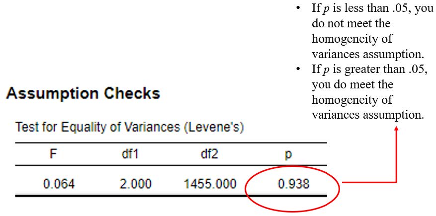
To interpret the results of the Levene’s test, we need to look at the significance or probability value. If p is less than .05, the test is significant, and we do not have homogeneity of variances. If p is greater than .05, the test is non-significant, and we do have homogeneity of variances. Because our p value is .94, which is greater than .05, we meet this assumption.
- If homogeneity of variances was met, you can proceed with interpreting the omnibus test without any homogeneity corrections.
To report the results of the Levene’s test in APA format, it might look something like this:
There was homogeneity of variances between groups, as assessed by the Levene’s test for equality of variances (p > .05).
Interpreting the Statistical Significance of the One-Way ANOVA Omnibus Test
The first thing we will interpret is the statistical significance of the omnibus test. To do this, we will look at the ANOVA table in the output. Because we have homogeneity of variances, we can interpret this without any homogeneity corrections as shown in the first row of this table.
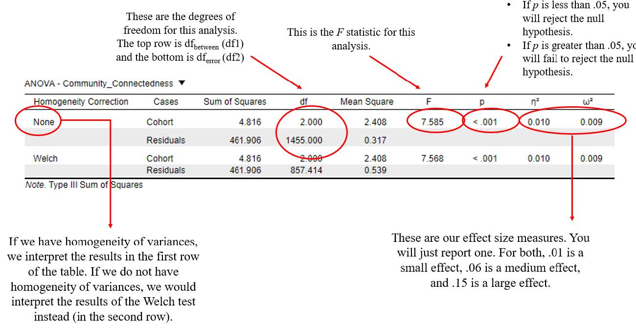
To interpret the results, we want to look at the p value. If p is less our alpha level of .05, we will reject the null hypothesis (indicating there is a significant statistical difference between the means of the groups on our dependent variable). If the p value is greater than our alpha level of .05, we will fail to reject the null hypothesis (indicating there is not a significant statistical difference between the group means on our dependent variable).
In this example, you can see that our p value is <.001, which is less than the alpha of .05. Therefore, we will reject our null hypothesis – there is at least one significant group mean difference on connection with the LGBT community between the younger, middle, and older cohorts.
Writing the basic results of the omnibus ANOVA test (F test) in APA format follows this general format:
F(df1, df2) = F statistic, p < .05 or p > .05, η2 = η2 value OR ω2 = ω2 value
So, plugging in our results into this format should look like this:
F(2, 1455) = 7.59, p < .05, η2 = .01 OR ω2 = .01
Now that we know we have a significant difference between the mean levels of community connectedness between our three conditions, what does this mean? Which of the conditions, specifically, are different from one another in regard to community connectedness? To answer these questions, we will need to look at the Post Hoc Analyses section.
Post Hoc Analyses: Community Connectedness
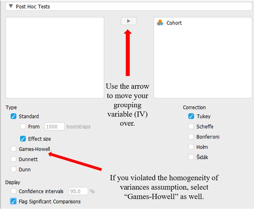
Now that we have rejected our null hypothesis and determined there is at least one age group that is significantly different in their level of connection to the LGBT+ community, let’s conduct post hoc tests to determine what groups are different. Post hoc analyses allow us to understand which of our groups/levels of the independent variable are different from one another. To do this, go back to the ANOVA test selection for the community connectedness outcome variable. Under “Post Hoc Tests” we will move our grouping variable [Cohort] over using the arrow and select:
- Under Type: select ‘Standard’ and ‘Effect size’ (Note: If we had violated the homogeneity of variances assumption, we would need to select the “Games-Howell” option here.).
- Under Correction: select ‘Tukey’
- Under Display: select ‘Flag significant comparisons’
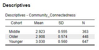
Which of our groups are significantly difference from one another? To examine this question, let’s look at both the “Descriptives” table and the “Post Hoc Tests” table from our output. The Descriptives table includes means, standard deviations, and sample size for each of our conditions. The Post Hoc Tests table details the results of all possible comparisons between our three groups.
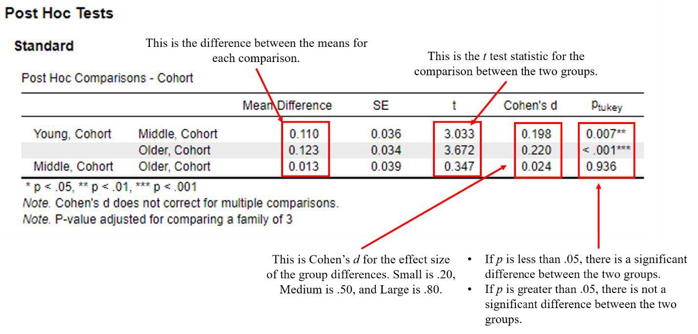
The Tukey post hoc test is a good one to select if you haven’t violated the homogeneity of variances assumption and you want to compare all possible combinations of group differences. The Post Hoc Tests table tells us not only whether the mean differences between the groups are statistically significant, they also tell us the effect size of this group difference by providing Cohen’s d. For each row in the table above, there is a test of the comparison between each group and the reference group (located on the far left). For instance, let’s look at the first two rows, each of which compare a given condition to the ‘control’ condition. Row one is the comparison between the means of the ‘younger’ group and the ‘middle group’; row two is the comparison between the means of the ‘younger’ group and the ‘older’ group; row three is the comparison between the mean of the ‘middle’ group and the ‘older’ group.
The information in the table above has the following meaning:
- Mean Difference – the mean difference between the reference group (‘younger’) and the target group (‘middle’), mathematically, it is Myounger – Mmiddle.
- Standard Error (SE) – the standard error of the mean difference between the reference group (‘younger’) and the target group (‘middle’)
- t – the test statistic from the independent measures t test comparing the reference group (‘younger’) and the target group (‘middle’)
- Cohen’s d – the Cohen’s d effect size for the comparison between the reference group (‘younger’) and the target group (‘middle’). This is interpreted the same as we’ve seen before.
- pTukey – The statistical significance level of the mean difference between the reference group (‘younger’) and the target group (‘middle’) Notice that the p value says Tukey next to it, indicating that these p values are corrected or adjusted for the number of comparisons that we could possibly run. Therefore, this p value accounts for the fact that we had three separate two-group comparisons.
From here, we would interpret the statistical and practical significance of each group pair comparisons. For each group comparison that was statistically significant, we would provide information using the following format, ending with “no other groups comparisons were significantly different, all pTukey > .05”:
Group 1 was [higher/lower] in DV (M = ?, SD = ?) compared to Group 2 (M = ?, SD = ?), pTukey < .05, d = Cohen’s d value, indicating a [small/medium/large group] difference. No other group comparisons were significantly different, all pTukey > .05.
If there were significant group differences between all of the groups, we could write something using the following format:
All groups were significantly different from one another (p tukey < .05). Group 1 reported the highest DV (M = ?, SD = ?), which was significantly higher than Group 2 (M = ?, SD = ?), p < .05, d = Cohen’s d value, and significantly higher than group 3 (M = ?, SD = ?), p < .05, d = ?. The difference between group 2 and group 3 was also significant (p < .05, d = ?).
If we were reporting in APA format using this formula, we would write the following:
The younger cohort was significantly higher in community connectedness (M = 3.03, SD = .56) compared to the older cohort (M = 2.91, SD = .57), pTukey < .05, d = .21, indicating a small-to-moderate group difference. The younger cohort was significantly higher in community connectedness (M = 3.03, SD = .56) compared to the middle cohort (M = 2.92, SD = .56), pTukey < .05, d = .20, indicating a small-to-moderate group difference. No other group comparisons were significantly different, pTukey > .05.
Primary Analyses: Omnibus Test for Life Satisfaction
Now let’s repeat the above steps, but for our second dependent variable or factor, ‘life satisfaction.’ Spoiler alert: We are running another set of analyses so we can practice how to handle violations to the homogeneity of variances assumption.
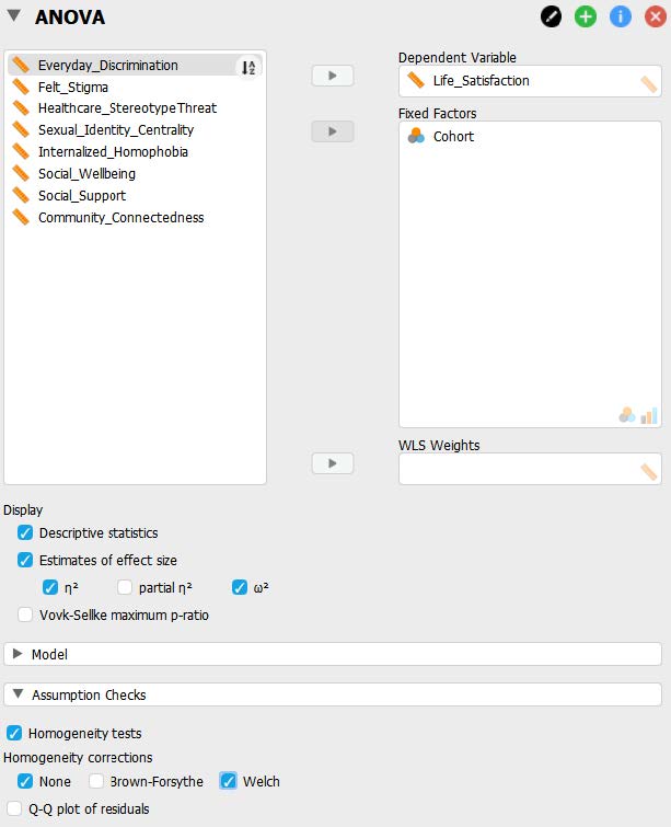
- First, we need to move our dependent variable [life satisfaction] to the “Variables” box and our independent variable [cohort] to the “Fixed Factors” box. We are then going to ask JASP to run the various analyses we will need to interpret for our test by clicking on the appropriate boxes in the window.
- Under “Display” we will want to check ‘Descriptive statistics’ and ‘Estimates of effect size’ – ‘eta- squared’ and ‘omega-squared’
- Under “Assumption Checks” select ‘Homogeneity tests’; under “Assumption corrections” select ‘None’ and ‘Welch’
Now that we have asked JASP to run the appropriate analyses for the omnibus test, let’s first look to see if we’ve met the assumption for homogeneity of variances. In your output, this is located under the “Assumption Checks” table and includes Levene’s test for equality of variances.
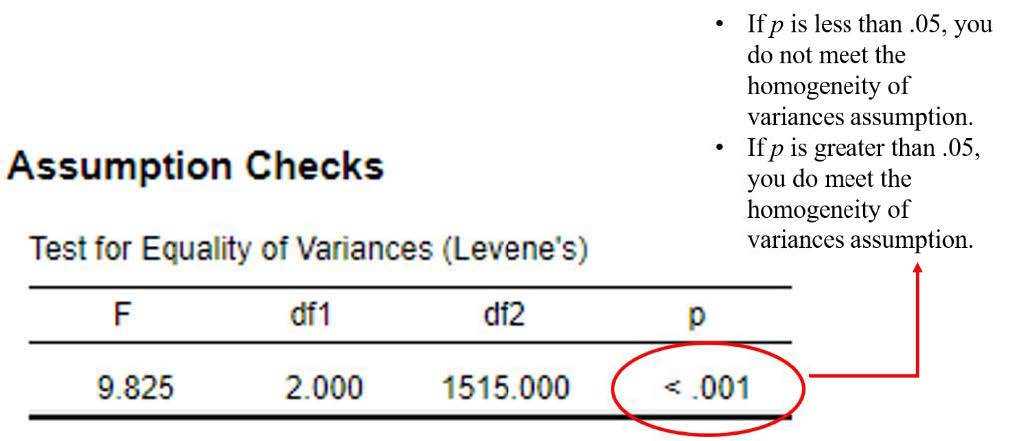
To interpret the results of the Levene’s test, we need to look at the significance or probability value. If p is less than .05, the test is significant, and we do not have homogeneity of variances. If p is greater than .05, the test is non-significant, and we do have homogeneity of variances. Our p value is <.001, which is less than .05. This means we do not meet this assumption.
- If homogeneity of variances was violated, you can continue conducting the one-way ANOVA, but will you need to have selected the “Welch” check box under ‘homogeneity corrections’ and interpret the “Welch” ANOVA results instead. As with independent measures t tests, the Welch homogeneity correction is calculated without pooling the variances. For this reason, it is often easier to select the “Welch” check box when running the omnibus test just in case the homogeneity assumption is violated. Additionally, if you violate the homogeneity assumption, there is an alternative post hoc selection which will be discussed in more detail in the Post Hoc Analyses section.
To report the results of the Levene’s test in APA format, it might look something like this:
There was not homogeneity of variances, as assessed by the Levene’s test for equality of variances (p < .05).
Interpreting the Statistical Significance of the One-Way ANOVA Omnibus Test
The first thing we will interpret is the statistical significance of the omnibus test. To do this, we will look at the ANOVA table in the output. Because we do not have homogeneity of variances, we interpret this with homogeneity corrections as shown in the second row in the table labeled ‘Welch’.
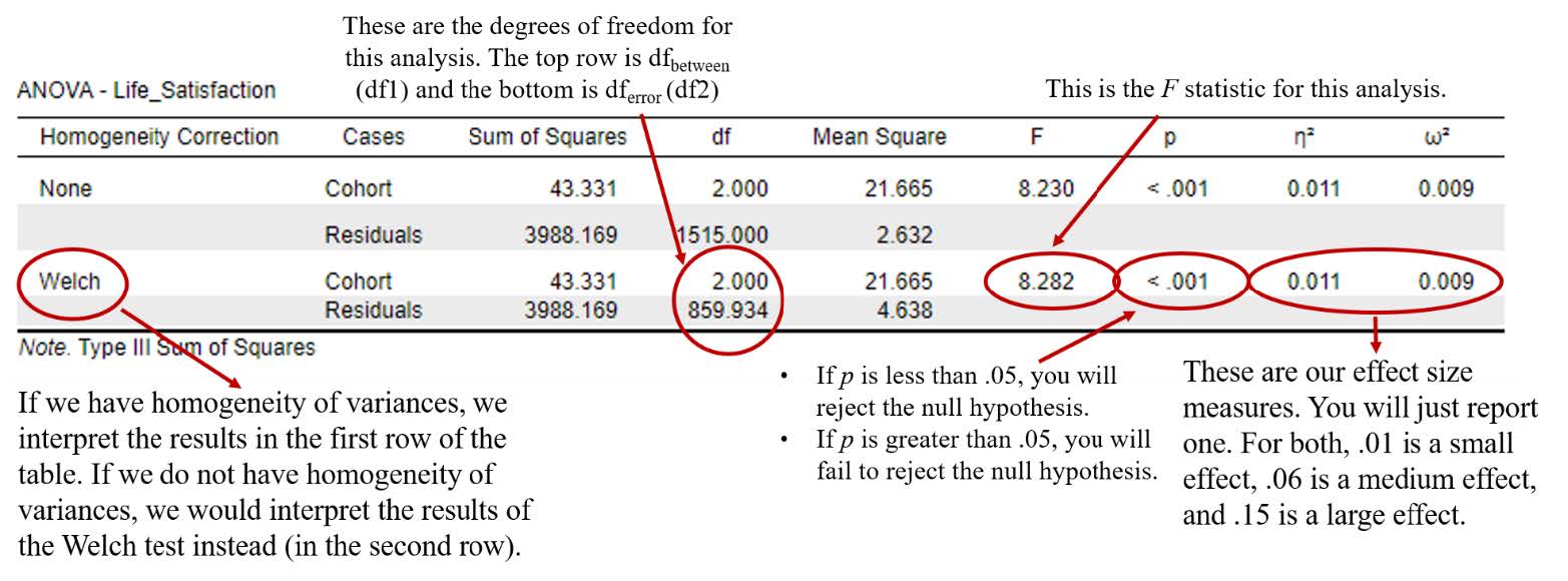
To interpret the results, we want to look at the p value. In this example, you can see that our p value is <.001, which is less than the alpha of .05. Therefore, we will reject our null hypothesis – there are significant group mean differences on life satisfaction between the younger, middle, and older cohorts.
Writing the basic results of the omnibus ANOVA test (F test) in APA format follows this general format:
F(df1, df2) = F statistic, p < .05 or p > .05, η2 = η2 value OR ω2 = ω2 value
So, plugging in our results into this format should look like this:
F(2, 859.93) = 8.28, p <.001, η2 = .01 or ω2 = .01
Now that we know we have a significant difference between the mean levels of life satisfaction between our three age groups, what does this mean? Which of the age groups, specifically, are different from one another regarding life satisfaction? To answer these questions, we will need to look at the Post Hoc Analyses section.
Post Hoc Analyses: Life Satisfaction
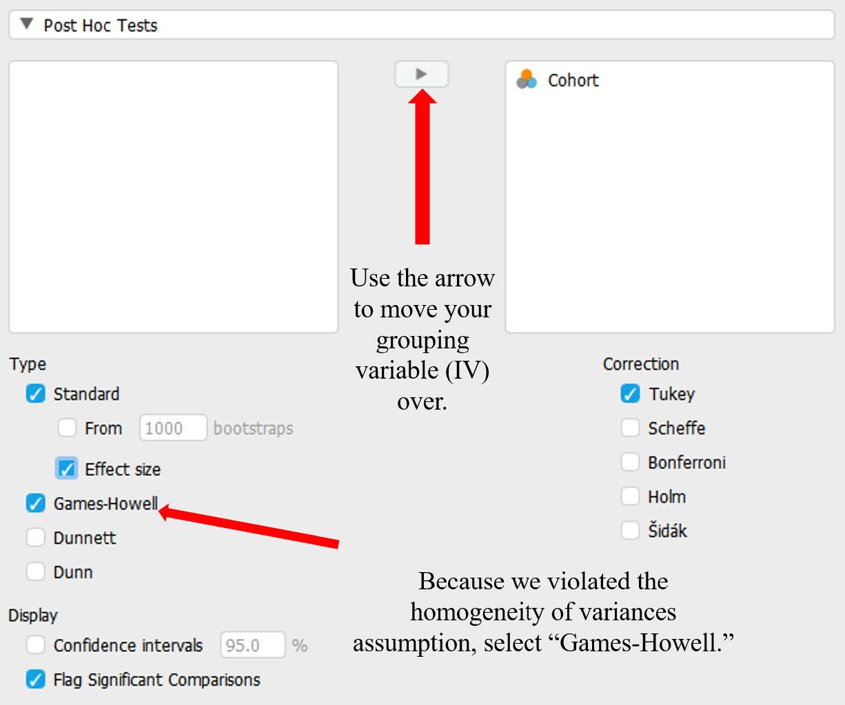
Now that we have rejected our null hypothesis and determined there is at least one age group that is significantly different in their level of life satisfaction, let’s conduct post hoc tests to determine what groups are different. To do this, go back to the ANOVA test selection for the life satisfaction outcome variable. Under “Post Hoc Tests” we will move our grouping variable [Cohort] over using the arrow and select:
- Under Type: select ‘Standard’ and ‘Effect size’ (Note: If we had violated the homogeneity of variances assumption, we would need to select the “Games-Howell” option here.).
- Under Correction: select ‘Tukey’
- Under Display: select ‘Flag significant comparisons’
Which of our groups are significantly difference from one another? To examine this question, let’s look at both the “Descriptives” table and the “Post Hoc Tests” table from our output.
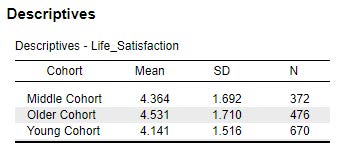
Looking at the preceding Descriptives table image, we can see the older cohort has the highest mean level of life satisfaction (M = 4.53), the middle cohort has the second highest mean level of life satisfaction (M = 4.36), and the young cohort has the lowest mean level of life satisfaction (M = 4.14). We still don’t know which groups are statistically different, but we can see a trend of the mean levels of life satisfaction increasing for each age group.
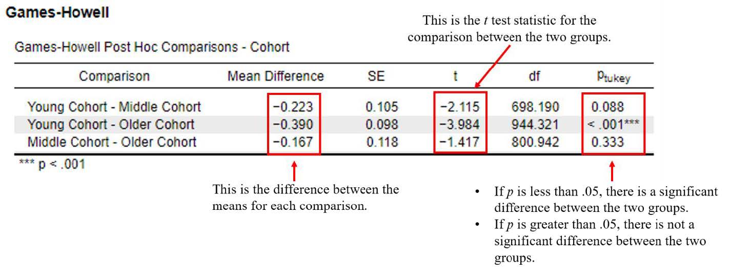
The Games-Howell post hoc test is preferred when your data violate the homogeneity of variances assumption. As you can see from the table above, it is set up a little differently than the Tukey post hoc test results. The Games-Howell Post Hoc Comparisons table still tells us if the mean differences between the groups are statistically significant; however, Cohen’s d effect size statistics are not available for this post hoc option. [Note: If you need to report an effect size for your post hoc comparisons, you can check the “Confidence Intervals” box under “Post Hoc Tests” and report the 95% confidence intervals for each comparison.] Unlike the tukey post hoc test table, the Games-Howell table tells us what groups are being compared in each row rather than using a reference group. The top row is comparing the young cohort and the middle cohort, the second row is comparing the young cohort and middle cohort, and the third row is comparing the middle cohort and the older cohort.
From here, we would interpret the statistical significance of each group pair comparisons. If we were reporting in APA format using this formula, we would write the following:
The older cohort (M = 4.53, SD = 1.71) had significantly higher levels of life satisfaction compared to the young cohort (M = 4.14, SD = 1.52), pTukey < .001. No other group comparisons were significantly different, pTukey > .05.
Interpreting the Practical Significance of the One-Way ANOVA Omnibus Test
Now that we have interpreted the statistical significance of our ANOVA Omnibus tests, let’s consider the practical significance. Remember, a significant p value tells us that there is a significant difference in the mean levels of community connectedness and life satisfaction between our three age groups. The effect size tells us how meaningful the difference between the age cohorts is for our dependent variable.
| n2 and w2 Effect Size Value | Strength |
| .01 | Small |
| .06 | Medium |
| .15 | Large |
Eta-squared (η2) or omega-squared (ω2) are both a representation of effect sizes for the omnibus test for an ANOVA. Because we are not yet able to say that, for example, Group 1 is different than Group 2 for the
omnibus ANOVA test, you have to estimate how much the difference is across all the groups. Therefore, eta- and omega-squared are used to determine the amount of variance accounted for (out of 100% variance) that the IV explains in the DV. These values are listed as proportions, so they never go over the value of one. To get this interpretation, we would multiply the value of eta-squared or omega-squared by 100 and interpret it as a percentage. In this example, therefore, we could say that 1.3% (eta-squared) or 1.1% (omega-squared) of the variance in community connectedness is accounted for by the experimental condition. Eta-squared is the more commonly reported effect size, while omega-squared is often used to help represent the true population effect size (Maxwell et al., 1981).
Let’s interpret eta-squared for our variables. We obtained eta-squared values of .01 – this is a small effect. So, although we have a statistical difference in the mean levels of community connectedness and life satisfaction between cohorts, that difference is small (negligible, even). This can often happen in studies that have a very large sample size. Finding a significant difference becomes easier, even if it is really small.
| Value (Notation) | |
| Omnibus Test | Test Statistic (F) |
| Degrees of Freedom (df1, df2) | Probability (p) |
| Assumptions | Skewness and Kurtosis |
| Boxplot | Levene’s Test |
| Post Hoc Analyses | Mean (M) |
| Standard Deviation (SD) | Probability of comparison (pTukey) |
| Effect Size (Cohen’s d) | Effect Size (Eta- or omega-squared) |
Putting it All Together
We ran the test for both community connectedness and life satisfaction, but for simplicity, let’s just look at the full write-up for the community connectedness analysis.
A one-way ANOVA was conducted to examine whether there were any mean differences in community connectedness between cohorts. There were outliers identified on community connectedness scores across conditions, as assessed by the inspection of a boxplot. We decided to retain these outliers given the large sample size and so as to avoid removing a large number of datapoints from the model. The scores on community connectedness were normally distributed across all conditions, as skewness and kurtosis statistics fell within the acceptable range of -2 and +2. There was homogeneity of variances, as assessed by the Levene’s test for equality of variances (p > .05).
The omnibus test was statistically significant, F(2, 1455) = 7.59, p < .05, η2 = .01 OR ω2 = .01. Post hoc analyses revealed that the younger cohort was significantly higher in community connectedness (M = 3.03, SD = .56) compared to the older cohort (M = 2.91, SD = .57), pTukey < .05, d = .21, indicating a small-to-moderate group difference. The younger cohort was also significantly higher in community connectedness (M = 3.03, SD = .56) compared to the middle cohort (M = 2.92, SD = .56), pTukey < .05, d = .20, indicating a small-to-moderate group difference. No other group comparisons were significantly different, pTukey > .05.
Real World Meaning
Now that the statistical jargon is out of the way – what do our results mean? We rejected the null hypothesis for community connectedness and found differences between the younger cohort and the middle/older cohorts. This means the younger cohort feels a stronger connection to the LGBT community compared to the middle and older cohorts; however, given the small effect size we obtained, this difference is may not be practically meaningful. We also rejected the null hypothesis for life satisfaction and found differences between the younger cohort and the older cohort. This means the older members of the LGBT community included in this study felt more satisfied with their life than the younger cohort.
Thinking back to Meyer and colleagues (2021) original hypothesis using minority stress theory, they measured other variables to address their original research question. Specifically, they thought the theory would mean that societal improvements in attitudes toward sexual minorities as well as increased legislative protections, would result in improved mental health outcomes for younger cohorts of sexual minorities in the United States. Certainly, younger cohorts’ feeling a greater connection to the LGBT community might suggest that is true as well. Unfortunately, the data did not support their hypothesis. If the data supported the minority stress theory, we would have found higher levels of life satisfaction in the younger cohort; however, we found the highest levels of life satisfaction in the older cohort. Looking across all the outcomes Meyer and colleagues analyzed, they found that younger cohorts reported more experiences with physical violence, sexual violence, and verbal abuse. They also reported higher levels of felt stigma and psychological distress.
References
Meyer, I. H. (2003). Prejudice, social stress, and mental health in lesbian, gay, and bisexual populations: Conceptual issues and research evidence. Psychological Bulletin, 129(5), 674–697. https://doi.org/10.1037/0033-2909.129.5.674
Meyer, I. H., Russell, S. T., Hammack, P. L., Frost, D. M., & Wilson, B. D. M. (2021). Minority stress, distress, and suicide attempts in three cohorts of sexual minority adults: A U.S. probability sample. PloS One, 16(3), e0246827–e0246827. https://doi.org/10.1371/journal.pone.0246827
Pew Research Center (2019). Majority of public favors same-sex marriage, but division persist. Retrieved from https://www.pewresearch.org/politics/2019/05/14/majority-of-public-favors-same-sex-marriage-but-divisions-persist/
The Office of Equity, Diversity, and Inclusion (2020). The Supreme Court bans employment discrimination towards sexual and gender minorities. Retrieved from https://www.edi.nih.gov/blog/news/supreme-court-bans-employment-discrimination-towards-sexual-and-gender-minorities
Authors
This guide was written and created by Ashlyn A. Moraine, Ruth V. Walker, PhD, Hannah J. Osborn, PhD, and Erin N. Prince.
Acknowledgements
We would like to thank Ilan H. Meyer, Stephen T. Russell, Phillip L Hammack, David M. Frost, and Bianca D. M. Wilson for making their data available through the Inter-university Consortium for Political and Social Research (ICPSR). Additionally, we appreciate Dr. Kristen Black’s edits and suggestions during the creation of this guide.
Copyright
CC BY-NC-ND: This license allows reusers to copy and distribute the material in any medium or format in unadapted form only, for noncommercial purposes only, and only so long as attribution is given to the creator.