
2 Running and Interpreting a Paired Samples t test in JASP
Kendra E. Scott; Dr. Hannah J. Osborn; Erin N. Prince; and Ruth Walker
Download Data Sets:
- JASP Data File Paired Samples t test
- CSV Data File Paired Samples t test
- JASP Data File Paired Samples t test (Outliers Deleted)
- CSV Data File Paired Samples t test (Outliers Deleted)
The Association of American Universities conducted a Campus Climate Survey on Sexual Assult and Misconduct in 2019. After surveying over 181,000 students across 33 colleges and universities, they found that 13% reported experiencing non-consensual sexual contact. With women and transgender students reporting significantly higher rates than men. One way that colleges and universities have been working to reduce rates of sexual assault is through educational programs that teach students how to intervene to prevent sexual assault. Researchers Banyard, Moynihan, and Plante (2007) created a bystander intervention program to prevent sexual assault on college campuses. In their research article, they present data demonstrating the efficacy of effectiveness of their intervention program.
To study the efficacy of the program, participants were separated into three different groups: a control group that did not attend a prevention program, a group that attended a one-session prevention program, and a group that attended a three-session prevention program. For our analyses, we are going to analyze the pre-and-post-test bystander self-efficacy scores for the 1-Session Program group.
Bystander self-efficacy was measured in this study using a 14-item measure of participant confidence to perform bystander behavior. Participants were asked to rate how confident they are that they can perform 14 different types of bystander behavior from 0 (“can’t do”) to 100 (“very certain can do”). Sample questions included items such as, “How confident are you that you could ask a stranger who looks very upset at a party if they are ok or need help?” Higher scores mean the participant was more confident in their ability to perform bystander behaviors. The pre-test variable name is “PreBSE” and the post-test variable name is “PostBSE.”
Hypotheses
The null hypothesis is:
- Conceptual H0: There is no significant difference in bystander self-efficacy scores for the One-Session Prevention Group before and after the bystander intervention program.
- Mathematical H0: The population mean difference on bystander self-efficacy scores before and after the bystander intervention program is equal to zero; MD = 0.
The alternative hypothesis is:
- Conceptual H0: There is significant difference in bystander self-efficacyscores for the One-Session Prevention Group before and after the bystander intervention program.
- Mathematical H0: The population mean difference on bystander self-efficacy scores before and after the bystander intervention program is not equal to zero; MD ≠ 0.
JASP Analyses
In order to run analyses, the first thing we need to do is open the data set we will be working with. To do this, open JASP and follow the steps below.
File → Open → Computer → Browse → Select the Paired Samples t Test Data (Banyard et al. 2007 Paired Samples t Test Data JASP) file wherever it’s saved on your computer.
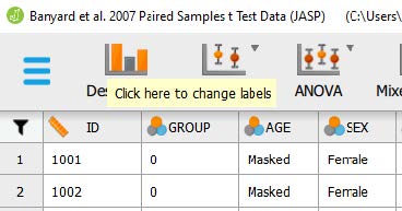
One the data set is open in JASP, we will change the data labels for our group variable so that we can select for those just in the 1-Session Program group. Currently the group column has a 0, 1, or a 2 for each participant. We will need to change these labels so that 0 = ‘control,’ 1 = ‘1-Session Program,’ and 2 = ‘3-Session Program.’ To change the numerical data into our categorical labels, you will take your cursor and hover over the ‘group’ column. When you see a note pop up saying, “click here to change labels” click on it. To change the labels, lick on the 0 under the Label column and type ‘control’. Then click on the 1 under the Label column and type ‘1-Session Program’. Then click on the 2 under the Label column and type ‘3-Session Program’. After you have changed the labels, you can close the window by clicking on the X button.
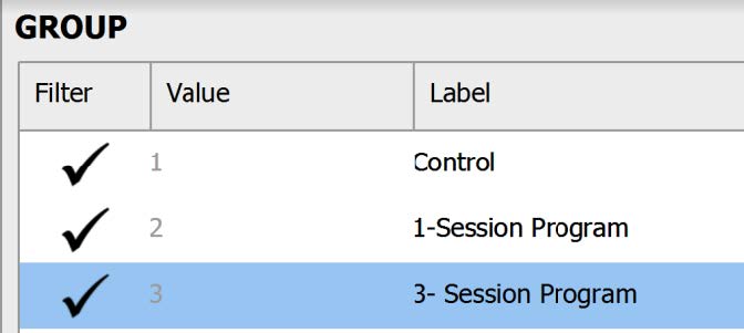
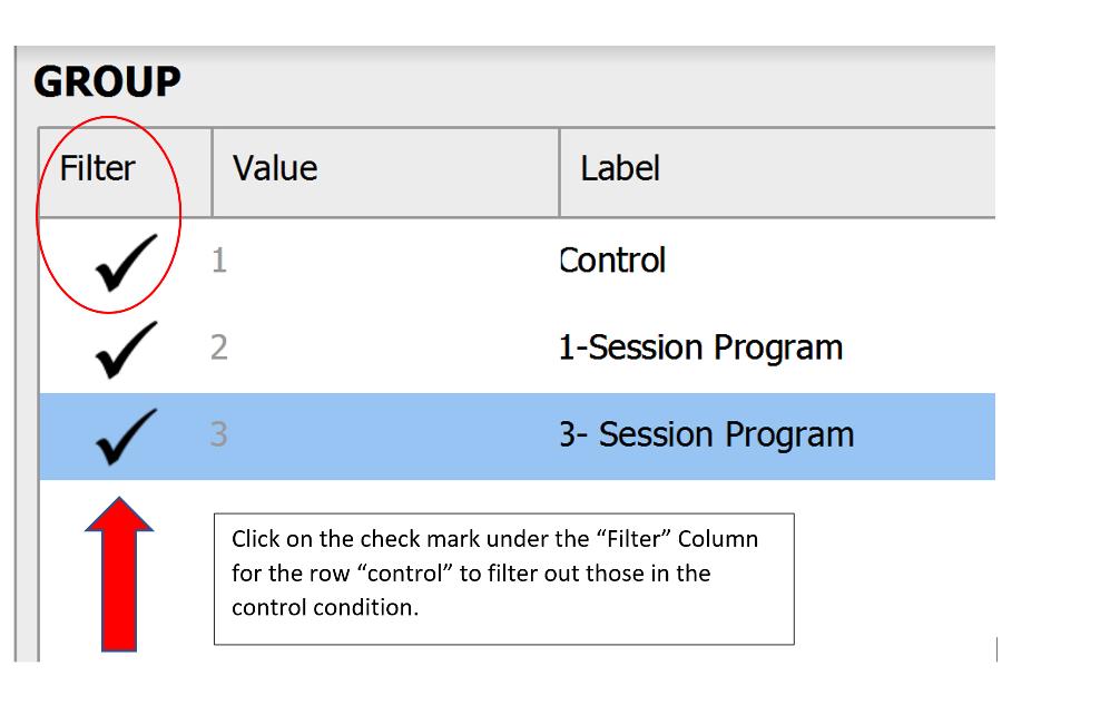
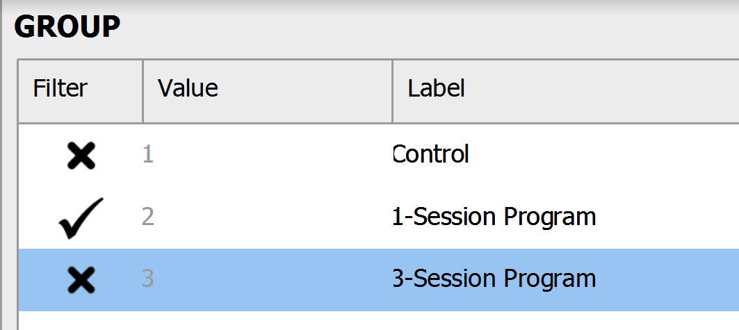
Before we test our assumptions, we also need to filter out participants who were in the control condition and 3- Session Program, so that we’re only looking at scores for those participants in the One-Session Program. One way to do this is to click on the Condition column to bring up the Values and Labels box. To filter out those in the control condition and Three-Session Program, under the “Filter” column, click the check mark – it will turn it into an X. Now, when we run any analysis, JASP will only consider those participants in the One-Session Program in the calculations!
Assumption Testing
Of the four assumptions, assumptions #3 and #4 must be tested prior to conducting a paired samples t test. Let’s consider whether our example data meets all four assumptions:
Assumption 1: Is there one dependent variable that is measured at the continuous (i.e., ratio or interval) level?
Yes. We have one dependent variable (bystander self-efficiency scores) and this dependent variable is a singular composite score of bystander self-efficiency based on 14 different types of bystander behaviors measured on a Likert-type scale. In psychological research, composite scores (i.e., averages of multiple individual questions) are treated as continuous data. Therefore, we meet this assumption.
Assumption 2: Is there one independent variable that consists of two categorical related groups or matched pairs?
Yes. We have a research design where each participant provides a score on the same dependent variable at two separate time points (before and after experiencing bystander intervention programs – “PreBSE” and “PostBSE.” in the dataset). Therefore, the scores are related across two (i.e., categorical) unique time points. Therefore, we meet this assumption.
Assumption 3: Are there any significant outliers in the difference scores between the two paired groups?
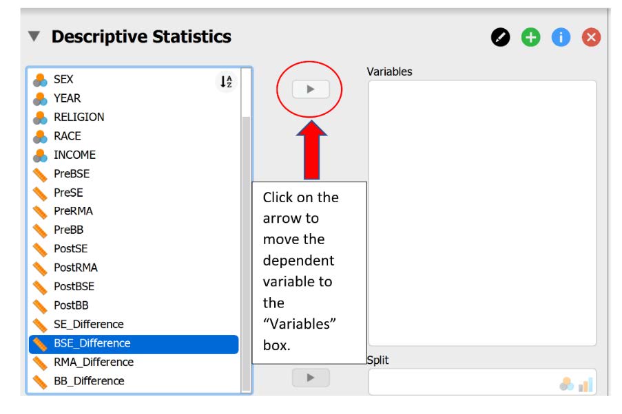
To check our data for Assumption 3 (and Assumption 4 to follow), we will be working with the Descriptives tab. When the “Descriptive Statistics” window pops up, we will need to move the difference score of our dependent variable (labeled “BSE_ Difference”) to the “Variables” box. This difference score was calculated by subtracting the pretest scores from the posttest scores on the dependent variable.
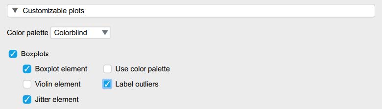
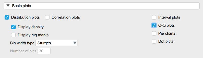
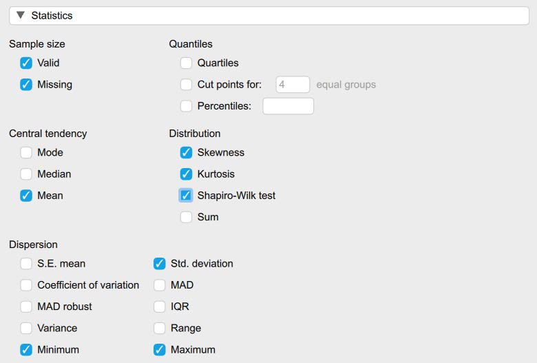
Then, under the “Customizable Plots,” “Basic Plots,” and “Statistics” tabs, select the following check marks.
- Under the “Customizable Plots” tab we will check the “Boxplots,” “Boxplot element,” “Jitter element,” and “Label outliers” boxes.
- We will also check “Distribution plots” and “Q-Q plots” under the “Basic plots” tab.
- Under the “Statistics” tab we will check the “Skewness,” “Kurtosis,” and “Shapiro-Wilk test” boxes.
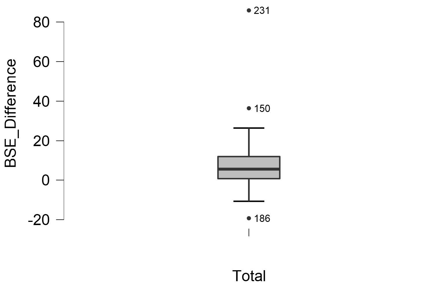
To determine if we have any outliers, we will look at the boxplots in our JASP output. If we have any outliers, they would be outside the top and bottom lines or whiskers. To help see the labeled outliers more clearly, you may want to uncheck the “jitter element” option. Looking at the boxplot below, we can see there are a total of 3 outliers labeled on the boxplot.
To report this is APA format, we would write:
There are 3 outliers in the difference scores for bystander self-efficiency, as assessed by the inspection of a boxplot.
Assumption 4: Is the distribution of the difference scores between the two related groups approximately normally distributed?
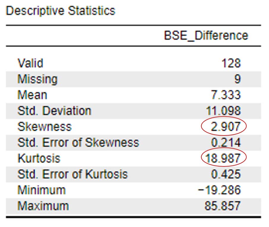
To determine if the difference scores for bystander efficacy are approximately normally distributed, we want skewness and kurtosis values between -2 and +2. Looking at the values on the output copied below, we can see our skewness statistic is not within the acceptable range of -2 and +2 (skewness: 2.91); additionally, our kurtosis statistic is a whopping 18.99! Neither of these statistics are within the acceptable range. Because normality is impacted by outliers, we may want to consider deleting the outliers to improve our normality statistics.
To report these results in APA format, we can write:
The difference scores for bystander self-efficacy were not normally distributed; skewness and kurtosis statistics were above the acceptable range of -2 and +2 at 2.91 and 18.99.
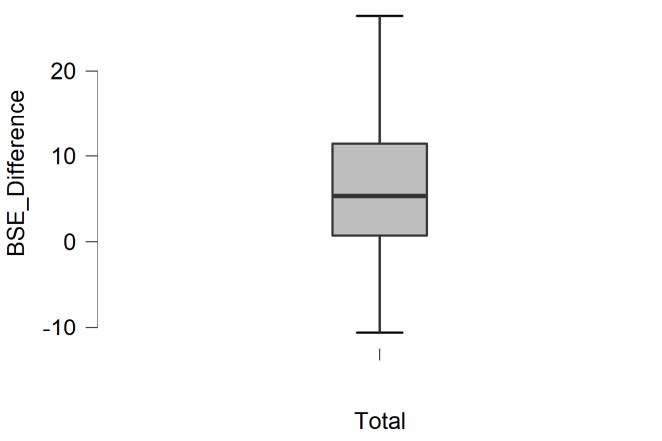
Let’s delete our outliers in order to meet our assumptions and recheck our assumptions. You can open the data file in Excel and delete the outliers yourself, or simply open the “Banyard et al. 2007 Paired Samples t Test Data Outliers Deleted JASP” file. Looking at our boxplot after deleting the 3 outliers, we can see there are no longer any outliers visible on our boxplot.
Rerunning our descriptive statistics, you can also see our skewness and kurtosis statistics have improved dramatically with the removal of the outliers and are now within the acceptable range of -2 and +2 at .36 (skewness) and -.26 (kurtosis).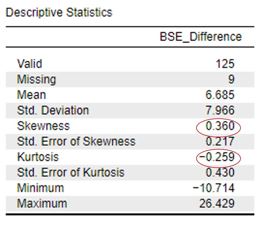
If you were writing these results up in APA formatting, you would want to let your readers know what you have done with your data (i.e., deleting outliers) and how that improved normality statistics. Researchers will sometimes report whether their primary analyses are different with the exclusion or inclusion of outliers in the dataset. In case you were wondering, the results of our analyses would be the same either way, but our data are normally distributed with the outliers deleted.
Primary Analyses
To run a paired samples t test, go to T-Tests at the top of the JASP screen and click on Paired Samples T-Test. We are going to conduct our primary analyses with the dataset that does not include the 3 original outliers, ‘Banyard et al. 2007 Paired Samples t Test Data Outliers Deleted (JASP).’
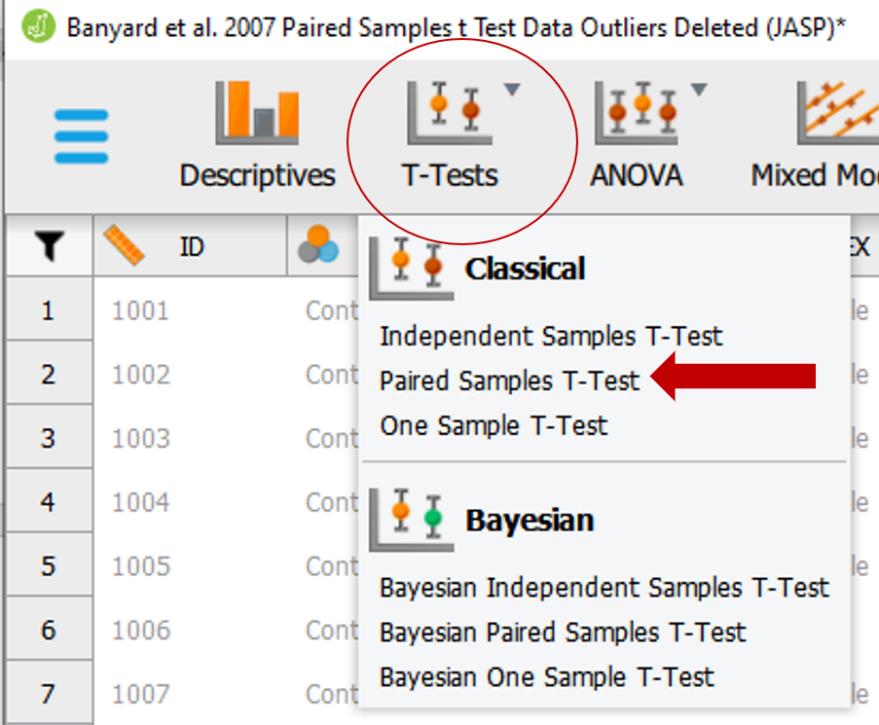
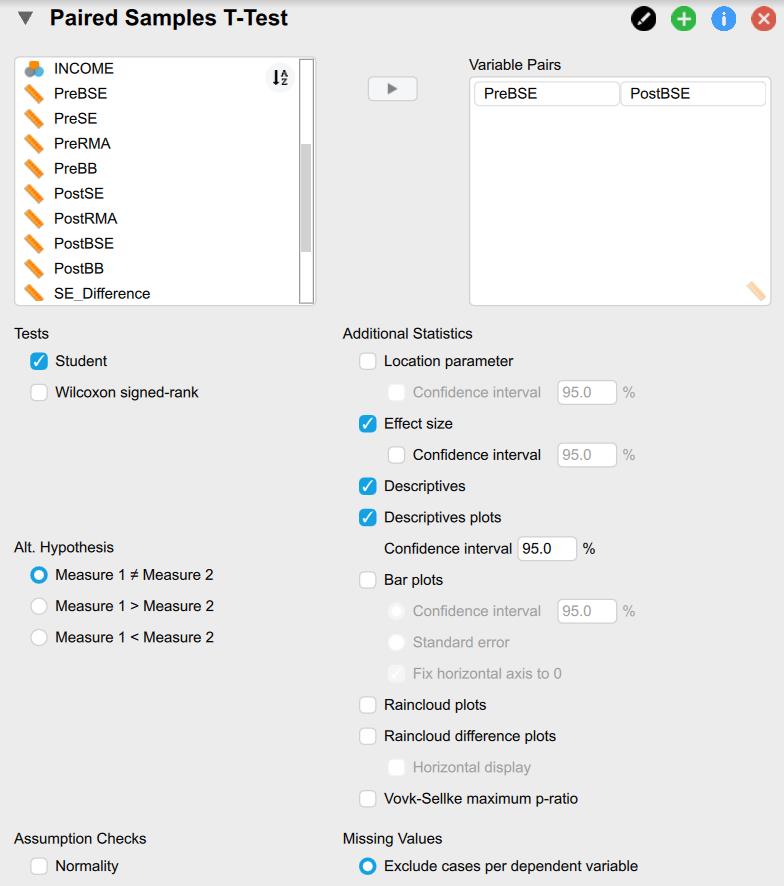
To run the paired samples t test, we need to move our two variable pairs (‘PreBSE’ and ‘PostBSE’) into the “Variable pairs” box. Then, we need to select the following check boxes as depicted in the image below:
- Tests: Student
- Additional Statistics: Effect Size, Descriptives, Descriptive Plots
Interpreting the Statistical Significance of Paired Samples t Tests
The first thing we will examine is the statistical significance of the paired samples t test. To do this, we are going to look at the “Paired Samples T-Test” table from the output.
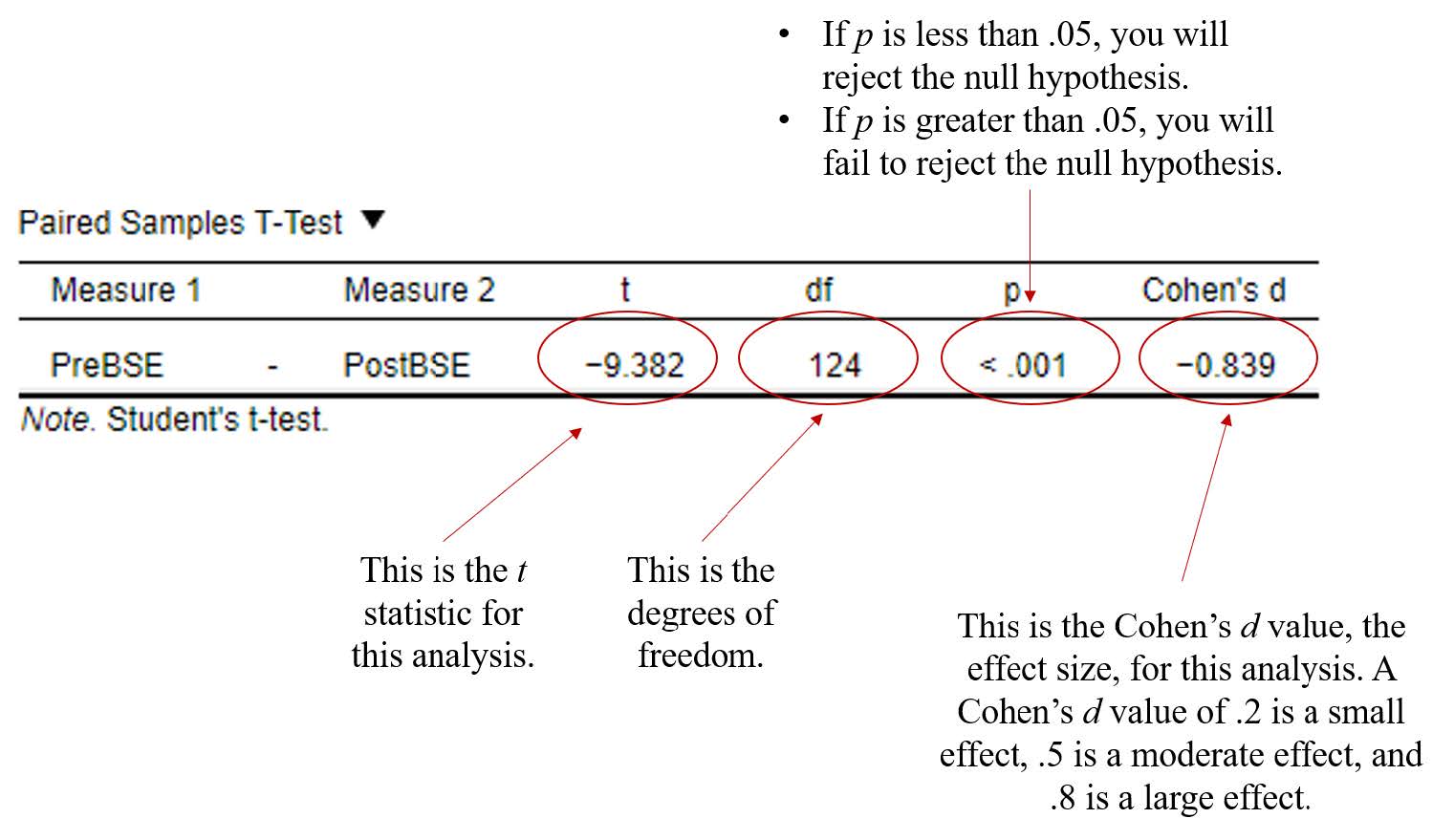
To interpret the results, we want to look at the p value. If p is less our alpha level of .05, we will reject the null hypothesis (indicating there is a significant statistical difference before and after the intervention on our dependent variable). If the p value is greater than our alpha level of .05, we will fail to reject the null hypothesis (indicating there is not a significant statistical difference before and after the intervention on our dependent variable).
In this example, you can see that our p value is <.001, which is less than the alpha of .05. Therefore, we will reject our null hypothesis – there is a significant difference in the bystander self-efficacy scores for One-Session Prevention Group before and after the bystander intervention program.
Writing the basic results of the t test in APA format following this general format:
t(df) = t statistic, p < .05 or p > .05, d = Cohen’s d statistic
Plugging in our results into this format should look like this:
t(124) = -9.38, p < .001, d = -.84
Now that we know there are significant statistical differences in the bystander self-efficacy scores for One-Session Prevention Group before and after the bystander intervention program – in what direction is this difference? Did people experience greater efficiency scores before, or after, the bystander intervention program? To answer this question, let’s look at the “Descriptives Table” and “Descriptive Plots” from our output to look at the means and standard deviations for our two groups of scores.
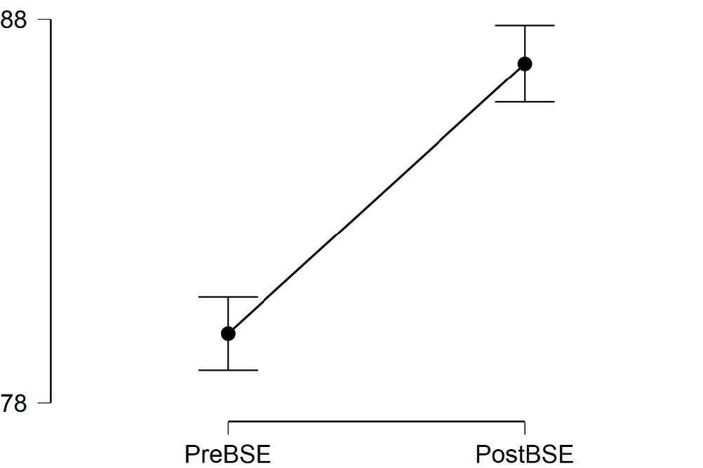
Remember, the descriptive plots provide a graphical representation of our results. This plot graphs the mean levels of bystander self-efficiency scores at time 1 (i.e., before the bystander intervention program) and at time 2 (i.e., after the bystander intervention program). By inspecting this graph, it is easy to see that participants reported higher scores of bystander self-efficiency after attending the bystander intervention program then before attending it.
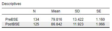
What we see visually from the Descriptives Plot is provided numerically in the Descriptives table. Provided in this table is information about sample size (N), means (Mean), standard deviations (SD) and standard errors (SE) for both groups of scores (i.e., at both time points). This table is important, because we will want to provide this information in the reporting of our results. Formatting this information into APA format, we might report the following:
A total of 124 individuals participated in this study and were in the 1- Session Program group. Participants reported significantly higher levels of bystander self-efficiency scores after (M = 86.84, SD = 11.92) as compared to before (M = 79.82, SD = 13.42) they attended the bystander intervention program.
Interpreting the Practical Significance of Paired Samples t Tests
Now that we have interpreted the statistical significance of the paired samples t test, let’s consider the practical significance of these results by looking at the effect size. Remember, a significant p value tells us that there is a statistically significant difference in self-reported bystander efficacy, but the effect size will tell us how large this difference actually is. Unlike p values, the Cohen’s d effect size measure is not impacted by sample size.
Cohen’s d Effect Sizes
| Effect Size | Strength |
| .2 | Small |
| .5 | Medium |
| .8 | Large |
The obtained Cohen’s d value in this example was -.84. Given that this value falls above the cut-off of .8 for a large effect, we would say that our results suggest a large effect. What this tells us is that not only are there statistically significant differences in bystander self-efficiency scores before and after attending a bystander intervention program to prevent sexual assault, but this difference is large. Meaning, after attending one-session of a sexual assault bystander intervention program, participants felt significantly more confident in their ability to intervene to prevent a sexual assault from happening.
Reporting in APA Format
What do you need to report in your results?
| Value (Notation) | Descriptives and Test Statistics |
| Mean (M) | Standard Deviation (SD) |
| Test Statistic (t) | Degrees of Freedom (df) |
| Effect Size | Cohen’s d |
| Assumptions | Skewness and Kurtosis |
| Boxplot |
Putting it All Together
A paired samples t test was conducted to determine if there were significant differences in bystander self-efficacy scores before and after attending a bystander intervention program. To correct for issues related to normality and outliers, three outliers were deleted from the dataset. The remaining data had no outliers, as assessed by the inspection of a boxplot and the difference scores for bystander efficacy were normally distributed, with skewness and kurtosis values within the acceptable range of -2 and +2. Participants reported significantly higher levels of bystander self-efficiency scores after (M = 86.84, SD = 11.92) as compared to before (M = 79.82, SD = 13.42) they attended the bystander intervention program, t(124) = -9.38, p < .001, d = -.84.
Real World Meaning
Recall that when we interpret the real world meaning of a study, we want to refrain from using any statistical jargon—that is to say, we want people who know nothing about statistics (a parent, your roommate, your friends, etc.) to be able to understand what the results of our statistical test are telling us about psychological phenomenon.
How would you describe the results of this study to someone who knows nothing about statistics? One thing that’s helpful is to think about what important pieces of information do we want to come across to the audience? In this example, we want to be able to communicate that the participants, reported higher scores of bystander self- efficiency scores after attending one session of a bystander intervention program compared to before attending one session. If I were describing the results of this study to my uncle, I would say the following:
Bystander intervention programs teach people ways they can stand up and help intervene to prevent sexual assault. Participants who attended one-session of a bystander intervention program felt more confident in their ability to act to prevent sexual assault after the program.
It should be noted that Banyard and colleagues (2007) conducted more complex analyses than what we cover in this course. The researchers included a Control Group and a 3-Session Intervention Group as well to establish a stronger experimental research design. They also measured participants across additional time points at 2-months, 4-months, and 12 months after the intervention. Because they also had multiple dependent variables they were interested in, the analyses they conducted were called a multivariance analysis of variance (MANOVA) to see if there were differences between the three conditions (i.e., control, one-session, and three-session groups). Additionally, they conducted repeated measures analysis to look at change over time, while controlling for participant gender by conducting a repeated measure multivariate analysis of covariance (MANCOVA). You will be very happy to know both of those analyses are beyond the scope of this class. 🙂
Overall, Banyard and colleagues (2007) found that participants in their one-and-three session groups reported significantly more knowledge of sexual violence, bystander attitudes, bystander behaviors, and bystander efficacy after attending the intervention. Additionally, they reported less rape myth acceptance. If you would like to learn more about bystander intervention programs, visit the National Sexual Violence Resources Center for more information.
References
Association of American Universities. (2019). AAU releases 2019 survey on sexual assault and misconduct. Retrieved from https://www.aau.edu/newsroom/press-releases/aau-releases-2019-survey-sexual-assault-and-misconduct
Banyard, V. L., Moynihan, M. M., & Plante, E. G. (2007). Sexual violence prevention through bystander education: An experimental evaluation. Journal of Community Psychology, 35(4), 463–481. https://doi.org/10.1002/jcop.20159
Authors
This guide was written and created by Kendra E. Scott, Ruth V. Walker, PhD, Hannah J. Osborn, PhD, and Erin N. Prince.
Acknowledgements
We would like to thank Victoria L. Banyard, Elizabeth G. Plante, and Mary M. Moynihan for making their data available through the Inter-university Consortium for Political and Social Research (ICPSR). Additionally, we appreciate Dr. Kristen Black’s edits and suggestions during the creation of this guide.
Copyright
CC BY-NC-ND: This license allows reusers to copy and distribute the material in any medium or format in unadapted form only, for noncommercial purposes only, and only so long as attribution is given to the creator.