
4 Running and Interpreting a One-Way Repeated Measures ANVOA in JASP
Ruth Walker and Matt C Cavanaugh
Download Data Sets:
Running and Interpreting a One-Way Repeated Measures ANVOA in JASP
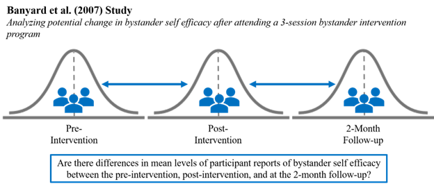
The Association of American Universities conducted a Campus Climate Survey on Sexual Assault and Misconduct in 2019. After surveying over 181,000 students across 33 colleges and universities, they found that 13% reported experiencing non-consensual sexual contact. With women and transgender students reporting significantly higher rates than men. One way that colleges and universities have been working to reduce rates of sexual assault is through educational programs that teach students how to intervene to prevent sexual assault. Researchers Banyard, Moynihan, and Plante (2007) created a bystander intervention program to prevent sexual assault on college campuses. This type of program teaches students to recognize situations that may be problematic and what methods they can use to intervene as an active bystander to stop sexual harassment and assault from happening. In their research article, the authors present data demonstrating the efficacy of effectiveness of their intervention program.
To study the efficacy of the program, participants were separated into three different groups: (1) a control group that did not attend a prevention program, (2) a group that attended a one-session prevention program, and (3) a group that attended a three-session prevention program. Participants in the treatment groups attended a 30-minute “booster” session two months following the initial intervention. Although Banyard and colleagues (2007) conducted For our analyses, we are going to analyze the data for the 3-Session Program group.
Rape Myth Acceptance was measured in this study using a 9-item measure of participant confidence they can do something to prevent violence. Participants were asked to rate how much they agree they can make a difference and help others on a 6-point likert scale from 1 (“completely disagree”) to 6 (“completely agree”). Sample questions included items such as, “I myself can make a difference in helping prevent violence.” Higher scores mean the participant was more confident in their ability to help prevent violence. The pre-test variable name is “PreRMA,” the post-test variable name is “PostRMA,” and the two-month follow-up variable is “2MORMA.”
Hypotheses
The null hypothesis is:
- Conceptual H0: There is no significant difference in Rape Myth Acceptances cores for the 3-Session Prevention Group before, immediately following, and two months after the bystander intervention program.
- Mathematical H0: The population mean difference on Rape Myth Acceptance scores for the 3-Session Prevention Group before, immediately following, and two months after the bystander intervention program is equal to zero; MD = 0.
The alternative hypothesis is:
- Conceptual H0: There is significant difference in Rape Myth Acceptance scores for the 3-Session Prevention Group before, immediately following, and two months after the bystander intervention program.
- Mathematical H0: The population mean difference in Rape Myth Acceptance scores for the 3-Session Prevention Group before, immediately following, and two months after the bystander intervention program is not equal to zero; MD ≠ 0.
JASP Analyses
In order to run analyses, the first thing we need to do is open the data set we will be working with. To do this, open JASP and follow the steps below.
Fileà OpenàComputeràBrowseà Select the One-Way Repeated Measures ANOVA Practice Data (Banyard et al., 2007) file saved on your computer.
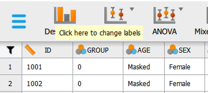
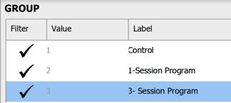
One the data set is open in JASP, we will change the data labels for our group variable so that we can select for those just in the 3-Session Program group. Currently the group column has a 0, X1, or a X2 for each participant. We will need to change these labels so that 0 = ‘control,’ X1 = ‘1-Session Program,’ and X2 = ‘3-Session Program.’ To change the numerical data into our categorical labels, you will take your cursor and hover over the ‘group’ column. When you see a note pop up saying, “click here to change labels” click on it. To change the labels, lick on the 0 under the Label column and type ‘Control’. Then click on the 1 under the Label column and type ‘1-Session Program’. Then click on the 2 under the Label column and type ‘3-Session Program’. After you have changed the labels, you can close the window by clicking on the X button.
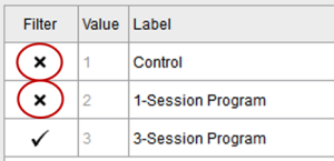
Before we test our assumptions, we also need to filter out participants who were in the control condition and 1-Session Program, so that we’re only looking at scores for those participants in the 3-Session Program. One way to do this is to click on the Condition column to bring up the Values and Labels box. To filter out those in the control condition and 1-Session Program, under the “Filter” column, click the check mark – it will turn it into an X. Now, when we run any analysis, JASP will only consider those participants in the 3-Session Program in the calculations!
Assumption Testing
Prior to conducting a one-way repeated measures ANOVA, we need to examine whether our data meets the first four assumptions:
Assumption 1: Is there one dependent variable that is measured at the continuous (i.e., ratio or interval) level?
Yes. We have one dependent variable (Rape Myth Acceptance) and this dependent variable is a singular composite score of self-reported self-efficacy based on 9 items measured on a Likert-type scale. Because composite scores are typically treated as continuous data in psychological research, we meet this assumption.
Assumption 2: Is there one independent variable that consists of one within-subjects factor with three or more categorical levels (e.g., one group of people measured across three time points)?
Yes. We have a research design where each participant provides a score on the same dependent variable across three separate time points: (1) pre-intervention, (2) post-intervention, and (3) 2-months post-intervention. Therefore, we meet this assumption.
Assumption 3: Are there any significant outliers in any of the levels of your independent variable?
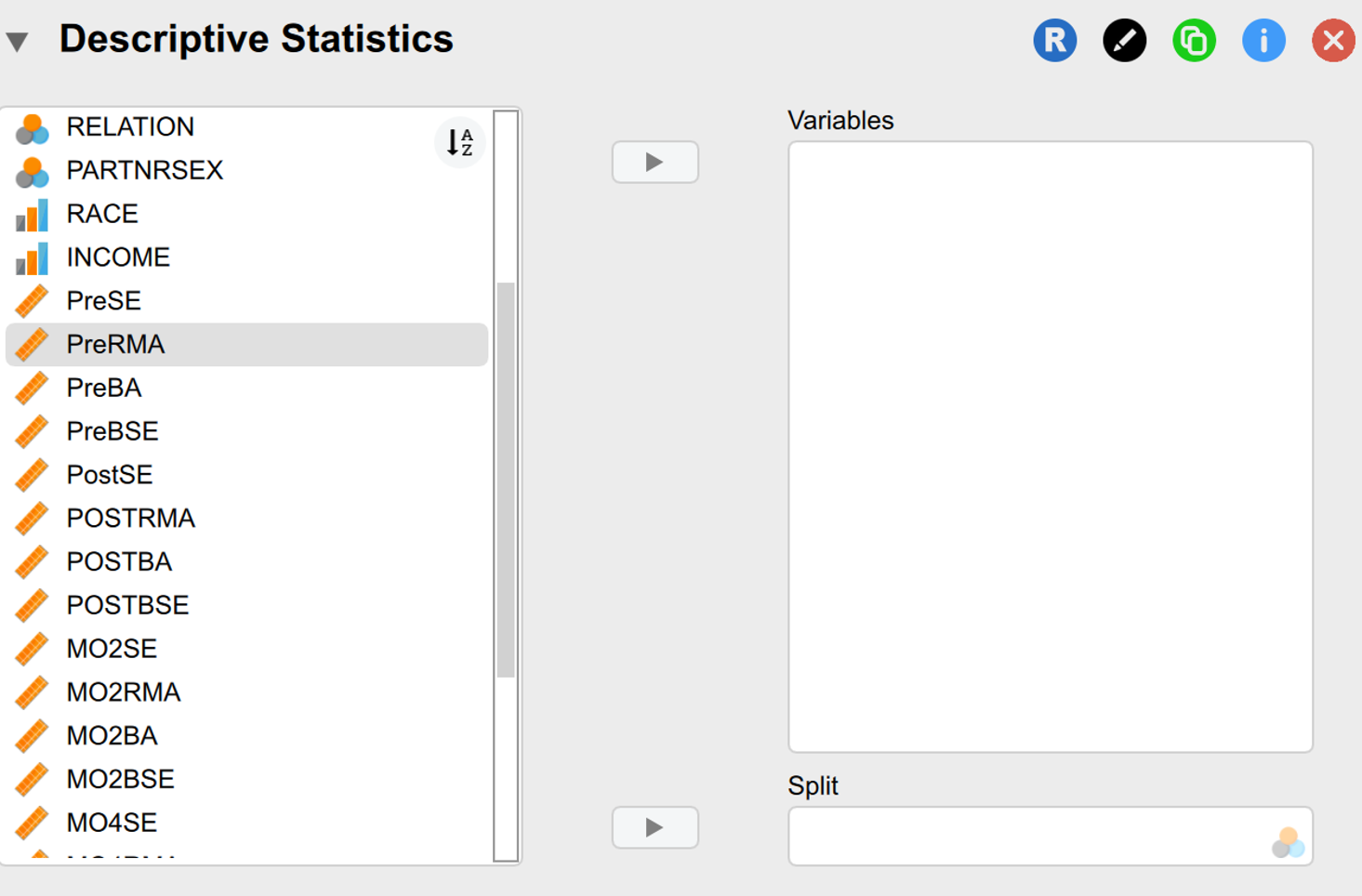
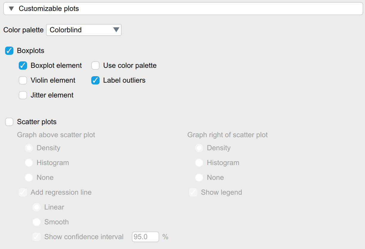
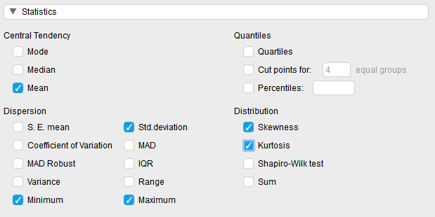
To determine if we meet this assumption, we will be using the Descriptives tab to see if there are any significant outliers in the boxplots across the three levels of our independent variable. To do this, we will click on the “Descriptives” button. When the “Descriptive Statistics” window pops up, we will need to move participant composite scores for self-efficacy before the intervention (“PreRMA”), immediately after the intervention (“PostRMA”), and two months after the intervention (“MO2RMA”) to the “Variables” box. Then, under the “Plots” and “Statistics” tabs, select the following check marks.
As with previous analyses, if we have outliers, we have to choose whether to include any outliers in our analyses, transform the dependent variable, or run a non-parametric equivalent instead (in this case, a Friedman test). It is generally best practice to run analyses with and without handling outliers to compare whether the results differ.
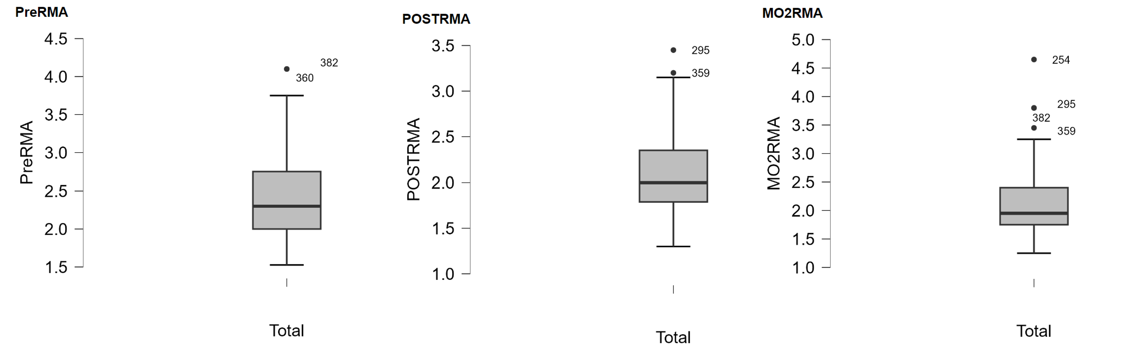
To determine if we have any outliers, we will look at the boxplots in our JASP output. If we have any outliers, they would be outside the top and bottom lines or whiskers. As you can see from the boxplot, we have two outliers in the top quartile of our time one measure of rape myth acceptance, two outliers in the top quartile of our time two (post intervention) measure of rape myth acceptance, and four outliers in our time three measure of rape myth acceptance. To report this is APA format, we would write:
There were two outliers in the pre-intervention measure of rape myth acceptance, two outliers post-intervention, and four outliers in the two-month follow up measure of rape myth acceptance, as assessed by the inspection of a boxplot.
Assumption 4: The dependent variable is approximately normally distributed for each level of the independent variable.
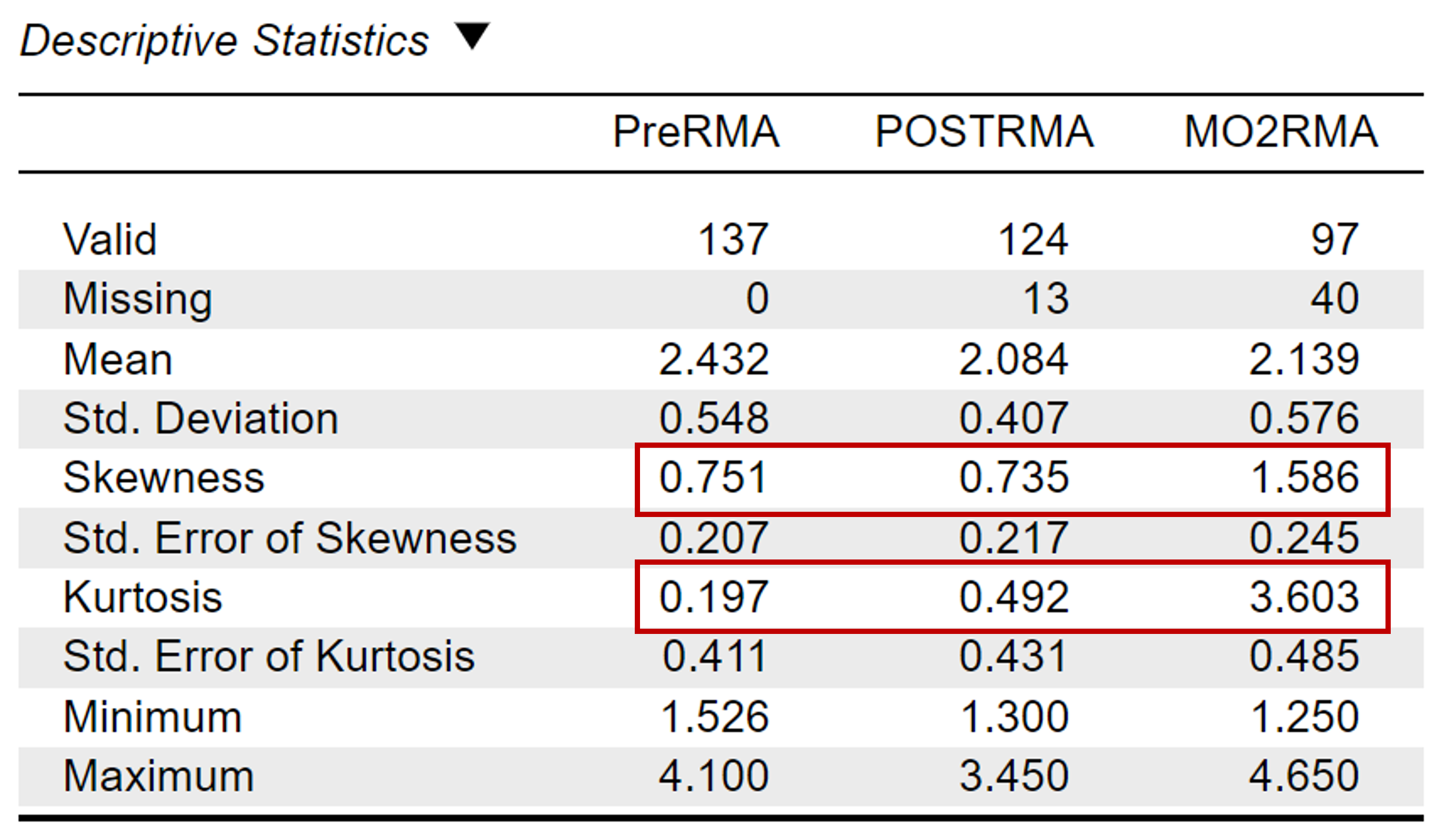
As with previous analyses, the assumption of normality is necessary for statistical significance testing using a one-way repeated measures ANOVA. To do this, we want to assess normality statistics (skewness and kurtosis values) across each time of measurement for our dependent variable. This means we will look at the normality statistics for self-efficacy before the intervention (“PreRMA”), after the intervention (“PostRMA”), and at the two-month follow-up (“MO2RMA”). We want all skewness and kurtosis values to be between -2 and +2. Looking at the values on the output copied below, we can see our skewness and kurtosis values for PreRMA, PostRMA, and MO2RMA. The difference scores are within the acceptable range of -2 and +2 (skewness: 0.75, 0.74, 1.59) (kurtosis: 0.2, 0.49, 3.60).
To report these results in APA format, we can write:
The scores for rape myth acceptance were normally distributed across all three time points, with all skewness and kurtosis statistics falling within the acceptable range of -2 and +2.
Assumption 5: The variances of the difference scores are approximately equal (also known as sphericity).
To check our last assumption, sphericity, we will need to run our primary analyses. Thus, we will come back to this assumption in the following section.
Primary Analyses
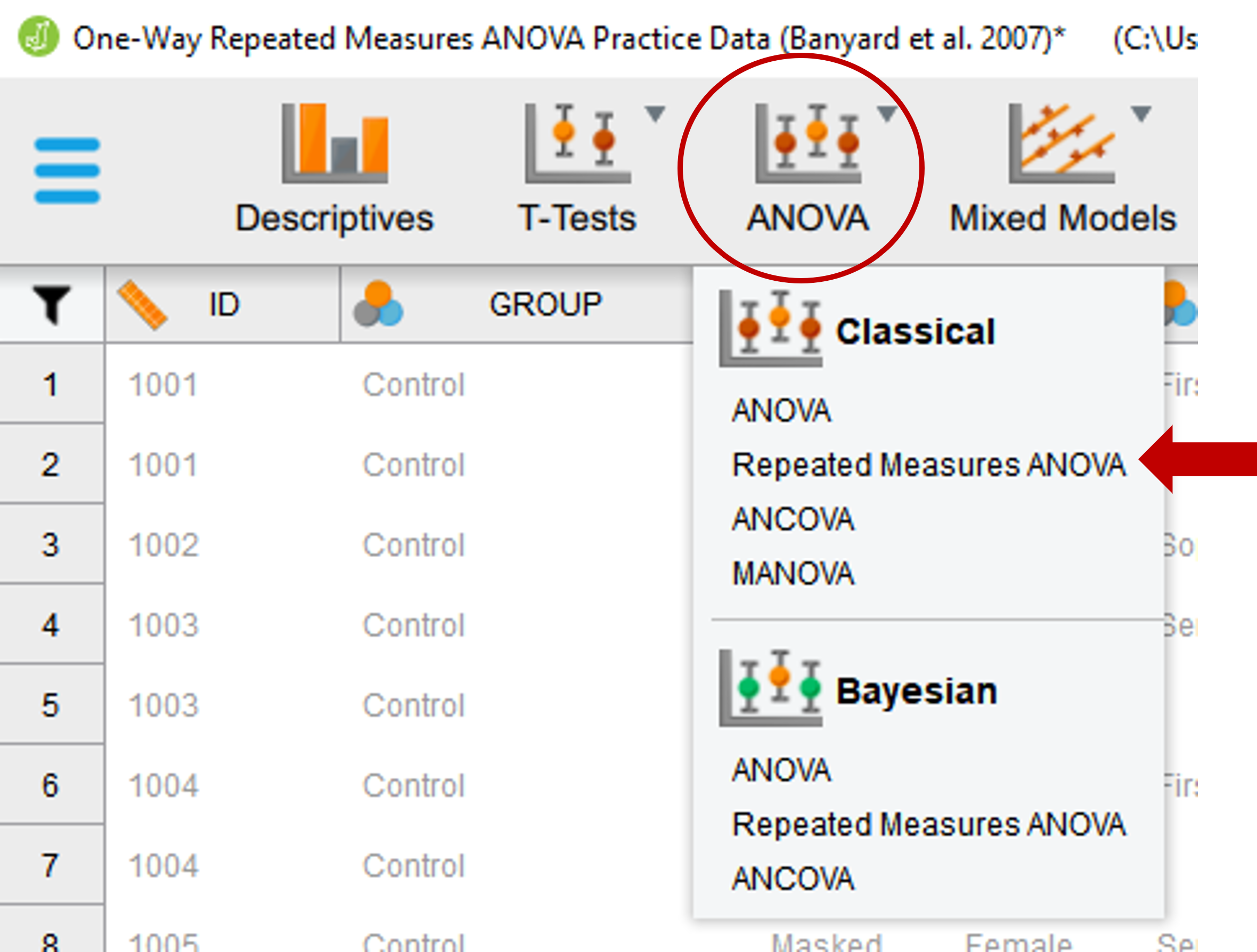
To run a one-way repeated measures ANOVA, go to ANOVA at the top of the JASP screen and click on Repeated Measures ANOVA.
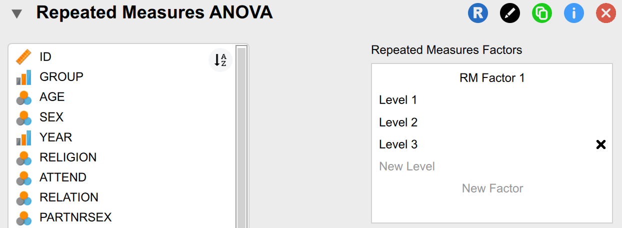
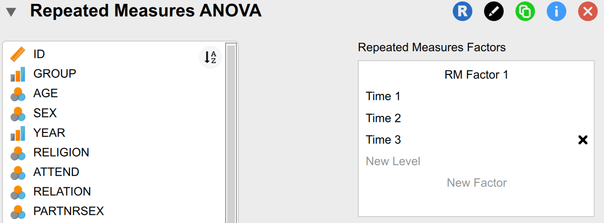
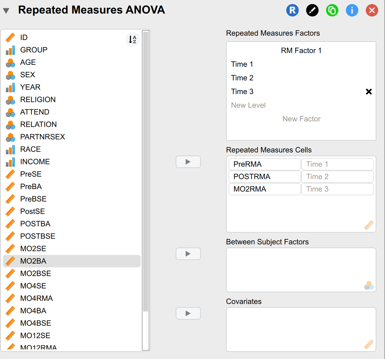
To run the repeated measures ANVOA, we need to label the levels of our independent variable or factor in the “Repeated Measures Factors” box. Since we are analyzing potential change across three time points, we will label the levels of our factor “Time 1,” “Time 2,” and “Time 3.”
Next, we need to move the three levels of our factor (“PreRMA,” “PostRMA,” and “MO2RMA”) into the “Repeated Measures Cells” box. We will move “PreRMA” next to the Time 1 label, “PostRMA” next to the Time 2 label, and “MO2RMA” next to the Time 3 label.
Then, we need to select the following check boxes:
- Display
- o Check the boxes for Descriptive statistics, Estimates of effect size, η2, and ω2.
- Assumption Checks
- o Check the boxes for Sphericity tests, Greenhouse-Geisser, Huynh-Feldt
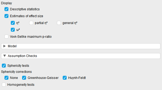
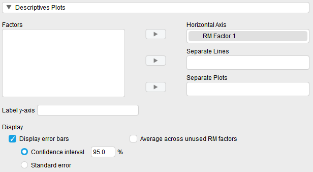
- Descriptives Plots: Move “RM Factor 1” to the “Horizontal Axis” box and check the “Display error bars” box
Assumption 5: The variances of the difference scores are approximately equal (also known as sphericity).
Now that we have begun running our repeated measures ANOVA, we want to look at our results to determine if we meet the sphericity assumption before we go any further. To do so, we will interpret Mauchly’s test of sphericity. Like the Levene’s test, we do not want the results to be significant. A p value less than .05 (p < .05) indicates that the Mauchly’s test is significant and you do not have sphericity. Alternately, a p value greater than .05 (p > .05) indicates that the Mauchly’s test is not significant and you do have sphericity.
- If the sphericity assumption is met, you can proceed with interpreting the omnibus test without any sphericity corrections.
- If the sphericity assumption is violated, you can continue conducting the repeated measures ANOVA, but will you need to check the “Greenhouse-Geisser” and “Huynh-Feldt” boxes under the “Assumption Checks” section. If sphericity estimates are .75 or greater, you will interpret the Huynh-Feldt correction. If sphericity estimates are less than .75, you will interpret the Greenhouse-Geisser correction. For this reason, it is often easier to check the “Greenhouse-Geisser” and “Huynh-Feldt” boxes when running the omnibus test just in case the sphericity assumption is violated.
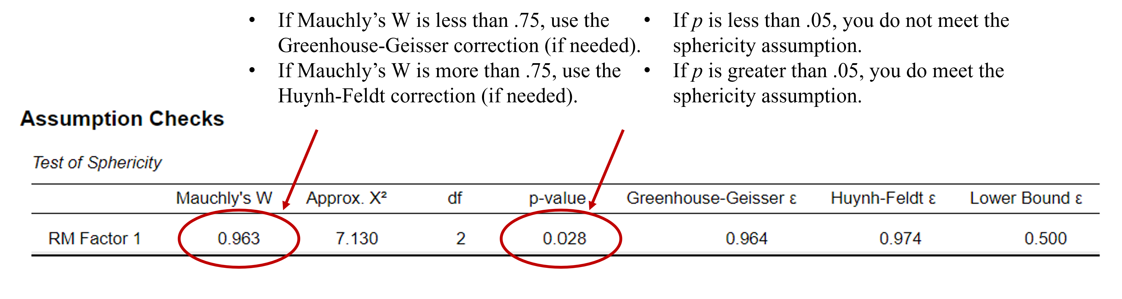
Looking at our Test of Sphericity results, we will look at our p-value first. Because our p-value is greater than .05, we then meet the sphericity assumption. Because of this, you can interpret sphericity with one of the statistical corrections that have been developed for this violation: Greenhouse-Geisser and Huynh-Feldt. To determine which correction we want to use, we need to look at the Mauchly’s W statistic. If this statistic is less than .75 you will interpret the Greenhouse-Geisser correction. If this statistic is more than .75, you will interpret the Huynh-Feldt correction. For the current analyses, the Mauchly’s W statistic is 0.96, so we will interpret the Hyunh-Feldt correction. You will notice adjusted degrees of freedom for time and error with the corrections in our omnibus test results.
To report the results of the sphericity test in APA format, it might look something like this:
The assumption of sphericity was violated (p < .05). The Mauchly’s W value was 0.96; thus, a Hyunh-Feldt correction was applied.
Interpreting the Statistical Significance of the Repeated Measures ANOVA Omnibus Test
The first thing we will interpret is the statistical significance of the omnibus test. To do this, we will look at the Repeated Measures ANOVA table in the output. Because the sphericity assumption has been violated, we will interpret the Hyunh-Feldt correction shown in the third row of the following table. If we did not violate the sphericity assumption, we would interpret the top row of the table labeled “None.”
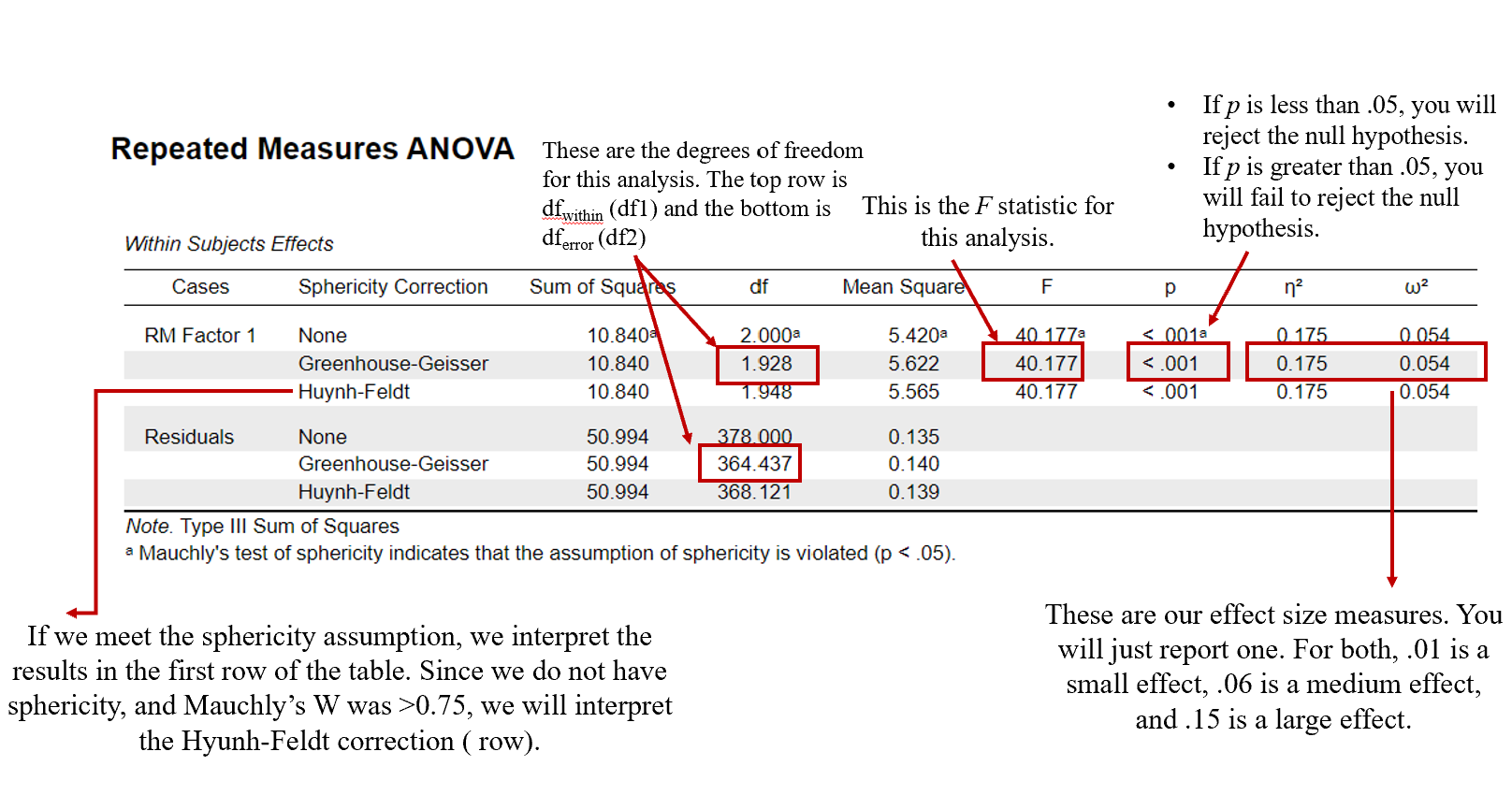
To interpret the results, we want to look at the p value. If p is less our alpha level of .05, we will reject the null hypothesis (indicating there is a significant statistical difference between self- endorsement of rape myth acceptance at one of the times of measurement). If the p value is greater than our alpha level of .05, we will fail to reject the null hypothesis (indicating there is not a significant statistical difference between participant self-endorsement of rape myth acceptance at one of the times of measurement).
In this example, you can see that our p value is <.001, which is less than the alpha of .05. Therefore, we will reject our null hypothesis – there is a significant difference in self- endorsement of rape myth acceptance at one of the times of measurement.
Writing the basic results of the Repeated Measures ANOVA in APA format following this general format (which will look familiar to the One-Way ANOVA):
F(df1, df2) = F statistic, p < .05 or p > .05, η2 = η2 value OR ω2 = ω2 value
So, plugging in our results into this format should look like this:
F(1.96, 188.23) = 28.3, p < .001, η2 = .08
Now that we know we have a significant difference between the mean levels of rape myth acceptance between the three times of measurement, what does this mean? Which of the times of measurement, specifically, are different from one another in regard to self-reported rape myth acceptance? Although we will be able to answer this question more accurately when we analyze and interpret the Post Hoc Analyses, let’s look at the estimated marginal means plots to gain a better understanding of what is happening with our data.

The descriptive plots provide a graphical representation of our results to help us visualize what is happening with our data. The preceding Descriptives Plots graphs the mean levels of Myth Acceptance at Time 1 (i.e., before attending the intervention), Time 2 (i.e., immediately after attending the intervention) and Time 3 (i.e., two months following the intervention). By inspecting this graph, it looks like there is a clear increase in reported Myth Acceptance before and after the intervention; however, the mean levels of Myth Acceptance at Time 3 look slightly lower than Time 2. Although we have to interpret our post-hoc tests to determine which time points are statistically different from one another, this gives us a general understanding of what is happening with self-efficacy across the three time points.
Interpreting the Practical Significance of Repeated Measures ANOVA Omnibus Test
Now that we have interpreted the statistical significance of the Repeated Measures ANOVA Omnibus test, let’s consider the practical significance of our results. The p value told us that there is a significant difference in the mean levels of rape myth acceptance between our three times of measurement. The effect size, then, tells us how meaningful the difference or change in rape myth acceptance is. That is, the effect size tells us how much the bystander intervention training is impacting scores on our dependent variable, rape myth acceptance.
Reminder: η2 and ω2 Effect Sizes”
| η2 and ω2 Effect Size Value | Strength |
| .01 | Small |
| .06 | Medium |
| .15 | Large |
Like the one-way ANOVA, eta-squared (η2) is the effect size for the omnibus test for a repeated measures ANOVA. Because we are not yet able to say that, for example, Time 1 is different than Time 2 for the omnibus test, you have to estimate how much the difference is across all times of measurement. Therefore, eta-squared is used to determine the amount of variance accounted for (out of 100% variance) that the IV explains in the DV. Remember, we can multiply the value of eta-squared by 100 to interpret these values as a percentage. In this example, we could say that 7.8% (eta-squared) of the variance in rape myth acceptance is accounted for by the bystander intervention. Eta-squared is the more commonly reported effect size, while omega-squared is often can be used to help represent the true population effect size (Maxwell et al., 1981).
We obtained an eta-squared value of .08 – this is a medium effect. This means that not only is there a statistically significant difference in participant rape myth acceptance across the three time points, but the difference in means levels of rape myth acceptance is moderate.
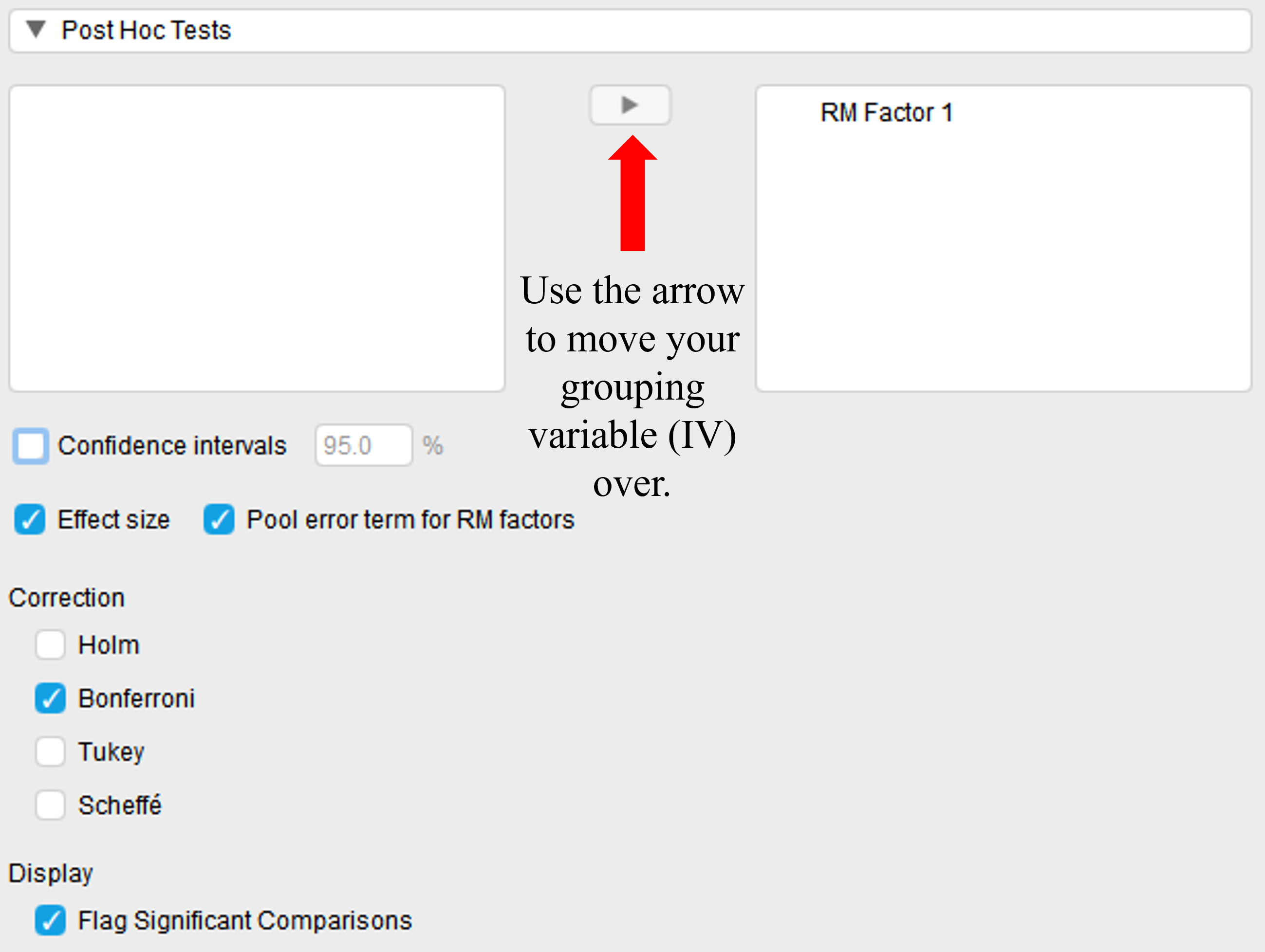
Post Hoc Analyses
Now that we’ve considered the statistical and practical significance of the repeated measures ANOVA omnibus test, let’s turn to post hoc analyses. These analyses allow us to understand which of our times of measurement are statistically different from one another. To do this, go back to the Repeated Measures ANOVA test selection in JASP. Under “Post Hoc Tests” we will move our factor “RM Factor 1” over using the arrow and check the boxes next to “Effect size,” “Bonferroni,” and “Flag Significant Comparisons.”
Which of our groups are significantly difference from one another? To examine this question, let’s look at both the “Descriptives” table and the “Post Hoc Tests” table from our output.
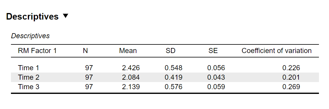
What we saw visually in the Descriptives Plot is provided numerically in the Descriptives table. Provided in this table is information about sample size (N), means (Mean), and standard deviations (SD) for all three times of measurement. This table is important, because we will want to provide this information in the reporting of our results. To understand whether there is a statistical difference between the mean values of rape myth acceptance across the three time points, we need to interpret the information provided in our Post Hoc Tests table.
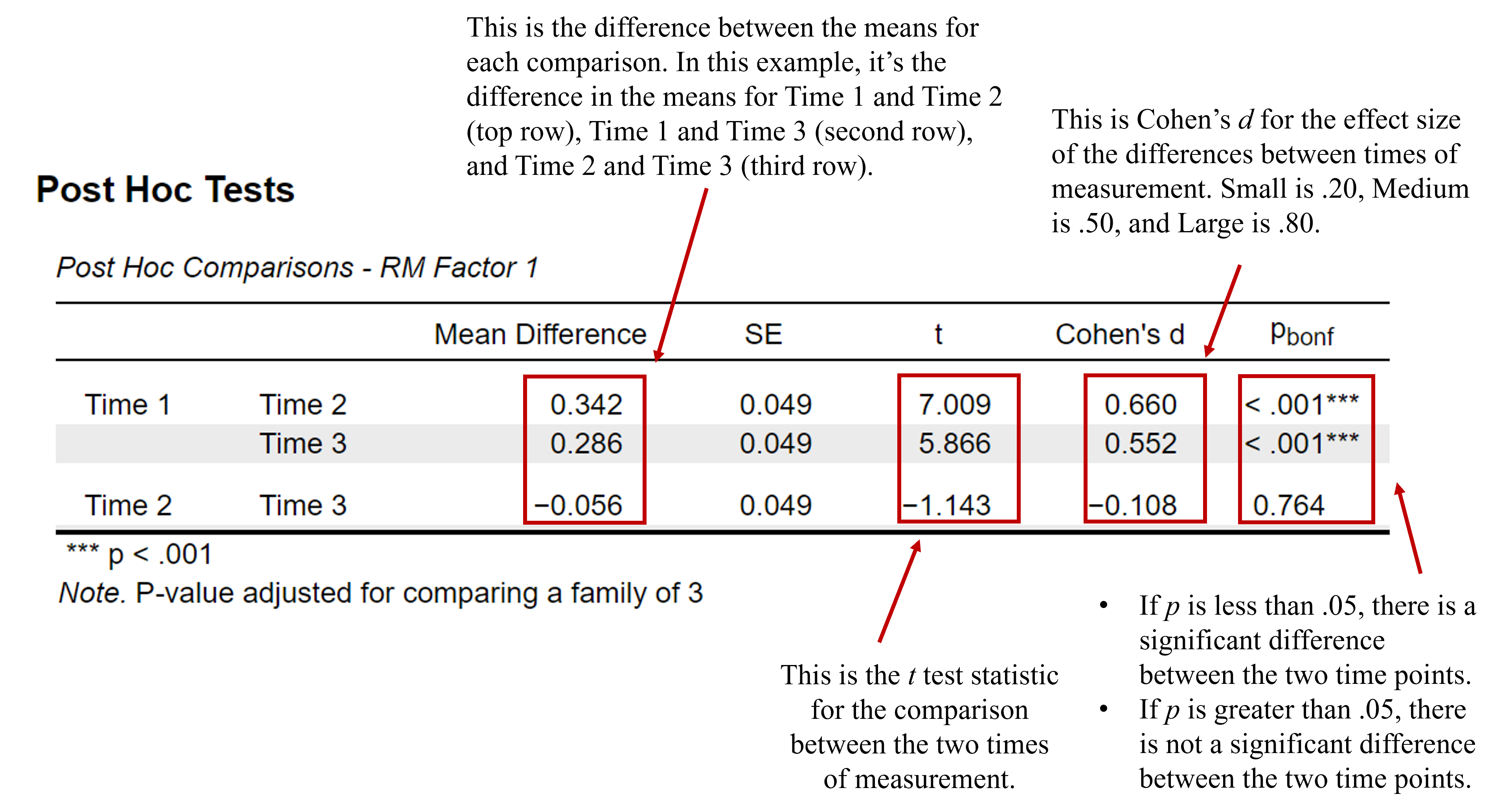
The Post Hoc Tests table tells us whether the mean differences between the mean values of rape myth acceptance across the three times of measurement are statistically significant. For each row in the table above, there is a test of the comparison between each time of measurement. The reference group is on the far-left column of the table. For instance, row one is the comparison between the mean levels of rape myth acceptance for Time 1 and Time 2; row two is the comparison between the means of Time 1 and Time 3; row three is the comparison between the means of Time 2 and Time 3.
The information in the table above has the following meaning:
- Mean Difference – the mean difference between the reference time point (Time 1) and the treatment time points after the intervention (Time 2 and Time 3). Mathematically, for example, it is MTime1 – MTime2.
- Standard Error (SE) – the standard error of the mean difference between the reference time point (Time 1) and the treatment time points after the intervention (Time 2 and Time 3).
- t – the test statistic from the independent measures t test comparing the reference time point (Time 1) and the treatment time points after the intervention (Time 2 and Time 3).
- Cohen’s d – the Cohen’s d effect size for the comparison between the reference time point (Time 1) and the treatment time points after the intervention (Time 2 and Time 3).
- Pbonf – The statistical significance level of the mean difference between the reference time point (Time 1) and the treatment time points after the intervention (Time 2 and Time 3). Notice that the p value says “bonf” next to it, indicating that these p values are corrected or adjusted for the number of comparisons that we could possibly run using a Bonferroni adjustment. Therefore, this p value accounts for the fact that we had three separate two-group comparisons.
From here, we would interpret the statistical and practical significance of each pair of comparisons. For each group comparison that was statistically significant, we would provide information using the following format, ending with “no other groups comparisons were significantly different, all pbonf >.05”:
Time 1 was [higher/lower] in DV (M = , SD = ) compared to Time 2 (M = , SD = ), pbonf < .05, d = Cohen’s d value, indicating a [small/medium/large group] difference. No other group comparisons were significantly different, all pbonf > .05.
If we were reporting in APA format using this formula, we would write the following:
Participant ratings of rape myth acceptance were significantly higher prior to attending the intervention (M = 2.43, SD = .55) compared to immediately after participants attended the 3-Session bystander intervention program (M = 2.00, SD = .41), pbonf < .001. Additionally, ratings of rape myth acceptance was also significantly lower prior to attending the intervention (M = 2.43, SD = .55) compared to when rape myth acceptance was measured two-months after participants attended the 3-Session bystander intervention program (M = 2.14, SD = .58), pbonf < .001, No other time comparisons were significantly different, pbonf > .05.
Reporting in APA Format
What do you need to report in your results?
| Value (Notation) |
| Omnibus Test |
| Test Statistic (F) |
| Degrees of Freedom (df1, df2) |
| Probability (p) |
| Effect Size (Eta- or omega-squared) |
| Assumptions |
| Skewness and Kurtosis |
| Boxplot |
| Mauchly’s Test of Sphericity |
| Post Hoc Analyses |
| Mean (M) |
| Standard Deviation (SD) |
| Probability of comparison (pTukey) |
| Effect Size (Cohen’s d) |
Putting it All Together
A one-way repeated measures ANOVA was conducted to examine whether there were any mean differences in student ratings of Rape Myth Acceptance before and after attending a 3-Session bystander intervention program. There were four outliers in the pre-intervention measure of self-efficacy, one outlier post-intervention, and no outliers in the two-month follow up measure of self-efficacy, as assessed by the inspection of a boxplot. We decided to retain these outliers given our results did not significantly differ when removed. The scores for rape myth acceptance were normally distributed across all three time points, with all skewness and kurtosis statistics falling within the acceptable range of -2 and +2. The assumption of sphericity was violated (p < .05). The Mauchly’s W value was 0.95; thus, a Hyunh-Feldt correction was applied.
The omnibus test was statistically significant, F(1.96, 188.23) = 28.3, p < .001, η2 = .08. Analyzing the post hoc comparisons using a Bonferroni correction, we found participant ratings of rape myth acceptance were significantly higher prior to attending the intervention (M = 2.43, SD = .55) compared to immediately after participants attended the 3-Session bystander intervention program (M = 2.00, SD = .41), pbonf < .001. Additionally, ratings of rape myth acceptance were significantly lower prior to attending the intervention (M = 2.43, SD = .55) compared to when rape myth acceptance was measured two-months after participants attended the 3-Session bystander intervention program (M = 2.14, SD = .58), pbonf < .001. No other time comparisons were significantly different, pbonf > .05.
Real World Meaning
Recall that when we interpret the real world meaning of a study, we want to refrain from using any statistical jargon—that is to say, we want people who know nothing about statistics (a parent, your roommate, your friends, etc.) to be able to understand what the results of our statistical test are telling us about psychological phenomenon.
How would you describe the results of this study to someone who knows nothing about statistics? One thing that’s helpful is to think about what important pieces of information do we want to come across to the audience? In this example, we want to be able to communicate that the participants, reported higher scores of self-efficiency or confidence to help prevent violence after attending three sessions of a bystander intervention program compared to before attending the program. This increase was maintained two months after they attended the program. If I were describing the results of this study to my uncle, I would say the following:
Bystander intervention programs teach people ways they can stand up and help intervene to prevent sexual assault. Participants who attended three sessions of a bystander intervention program felt more confident in their ability to act to prevent violence after the program. They continued to feel confident two months after attending the program.
It should be noted that Banyard and colleagues (2007) conducted more complex analyses than what we cover in this course. The researchers included a Control Group and a 1-Session Group as well to establish a stronger experimental research design. They also measured participants across additional time points at 4-months and 12 months after the intervention. Because they also had multiple dependent variables they were interested in, the analyses they conducted were called a multivariance analysis of variance (MANOVA) to see if there were differences between the three conditions (i.e., control, one-session, and three-session groups). Additionally, they conducted repeated measures analysis to look at change over time, while controlling for participant gender by conducting a repeated measure multivariate analysis of covariance (MANCOVA). You will be very happy to know both of those analyses are beyond the scope of this class. 🙂
Overall, Banyard and colleagues (2007) found that participants in their one-and-three session groups reported significantly more knowledge of sexual violence, bystander attitudes, bystander behaviors, and bystander efficacy after attending the intervention. Additionally, they reported less rape myth acceptance. If you would like to learn more about bystander intervention programs, visit the National Sexual Violence Resources Center for more information.
References
AAU releases 2019 survey on Sexual Assault and Misconduct | Association of American Universities (AAU). Association of American Universities. (2019, October 15). https://www.aau.edu/newsroom/press-releases/aau-releases-2019-survey-sexual-assault-and-misconduct
Banyard, V. L., Moynihan, M. M., & Plante, E. G. (2007). Sexual violence prevention through bystander education: An experimental evaluation. Journal of Community Psychology, 35(4), 463–481. https://doi.org/10.1002/jcop.20159
Maxwell, S. E., Camp, C. J., & Arvey, R. D. (1981). Measures of strength of association: A comparative examination. Journal of Applied Psychology, 66(5), 525–534. https://doi.org/10.1037/0021-9010.66.5.525
Authors
This guide was written and created by Ruth V. Walker and Matt C Cavanaugh. Please address any questions, concerns, or edits to Ruth Walker at ruth-walker@utc.edu
Acknowledgments
We would like to thank Victoria L. Banyard, Elizabeth G. Plante, and Mary M. Moynihan n for making their data available through the Inter-university Consortium for Political and Social Research (ICPSR).
Copyright
CC BY-NC-ND: This license allows reusers to copy and distribute the material in any medium or format in unadapted form only, for noncommercial purposes only, and only so long as attribution is given to the creator.