
8
Ruth V. Walker; Ashlyn A. Moraine; Kristen J. Black; Chloe Oberkirch; and Matt C Cavanaugh
Download Data Sets:
We are going to use a portion of the data that was used in the study by Li, Wu, and Xiong (2021). This is the same study we used when we conducted a Pearson Correlation in the previous guide and found a strong, positive relationship between employee levels of cultural intelligence (e.g., ability to adapt to cross-cultural environments) and their innovative behaviors in the workplace. For this guide, we will be building upon that analysis by first conducting a simple linear regression to determine if Cultural Intelligence predicts innovative behaviors in the workplace. As we learned in the previous guide, Sustainable Innovation Behavior refers to how well an individual creates and enacts new ideas.
The researchers measured Sustainable Innovation Behavior (SIB) by asking participants to answer six questions rated on a 7-point Likert scale. Higher scores on this scale indicate higher levels of Sustainable Innovative Behavior. A sample item includes, “I often come up with creative ideas.”
The researchers measured Cultural Intelligence (CQ) by asking participants to answer 12 questions rated on a 7-point Likert scale. Higher scores on this scale indicate higher levels of Cultural Intelligence. A sample item includes, “I adjust my cultural knowledge as I interact with people from a culture that in unfamiliar to me.
Now we are ready to try out an analysis of our own. Open up the “Li et al 2021” file. You have both a .csv file you can upload and a Jamovi file.
Hypotheses
We know there is a relationship between Cultural Intelligence and Sustainable Innovation Behaviors after completing a Pearson correlation; however, now we are going to build on those results to determine if Cultural Intelligence predicts Sustainable Innovation Behaviors using a linear regression model.
The null hypothesis is:
- Conceptual H0: Cultural Intelligence will not predict Sustainable Innovation Behavior.
- Mathematical H0: b = 0
The alternative hypothesis is:
- Conceptual H1: Cultural Intelligence will predict Sustainable Innovation Behavior.
- Mathematical H1: b≠ 0
Linear Regression Equation
Y′ = bX + a
Sustainable Innovative Behavior′ = (b x Cultural Intelligence) + a
Here is a breakdown of the components of the regression question:
- Y′ is the predicted value of your outcome or dependent variable (Y)
- b is the slope of the regression line (estimated by regression)
- May also be written using this symbol instead: ꞵ1
- X is the value of your predictor variable or independent variable
- a is the Y-intercept of the regression line (estimated by regression)
- May also be written using this symbol instead: ꞵ0
Jamovi has a range of add-on modules that can be activated which expand the analysis options available. One of these, the General Analyses for Linear Models in Jamovi, or gamlj module, will allow us to obtain our simple effects.
To add this package, click the blue plus sign labeled “Modules” in the top right corner of the Jamovi window.
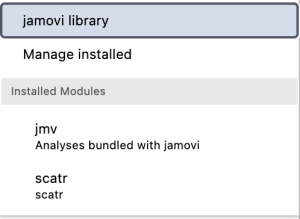
From the dropdown menu, select “Jamovi Library.”
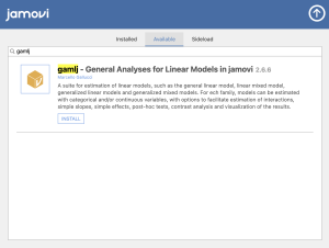
A window will appear, type “gamlj” in the search bar and click “Install” once you see this result.
Once you have installed the gamlj package, this new Linear Models option should appear in your analyses tab.

Assumption Testing
Let’s walk through testing all six of our assumptions.
Assumption One: Are our variables continuous?
Yes. Our predictor, Cultural Intelligence is a continuous variable measured using a 12-item Likert scale questionnaire. Our dependent variable is also a continuous variable measured using a 6-item Likert scale questionnaire.
Assumption Two: Are the variables normally distributed?
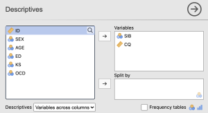
To continue our assumption testing, click Exploration then select “Descriptives” from the dropdown menu. When the “Descriptive Statistics” window pops up, we will need to move the following study variables to the “Variables” box on the right: Cultural Intelligence and Sustainable Innovation Behavior.
In the Statistics drop down menu, check the boxes next to Skewness and Kurtosis under Distribution.
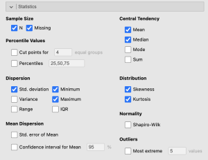
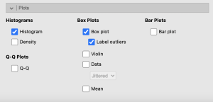
Under the Plots option select the following options:
- Histogram
- Box plot
- ○ Label outliers
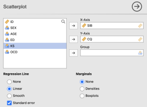
In order to create a scatterplot, select the “Scatterplot” option from the “Exploration” dropdown menu. Ensure that your variables of interest are both continuous, change them if not. Use the arrows to move your SIB and CQ variables into the X- and Y-Axis. Under “Regression Line”, select the ‘Linear’ and ‘Standard error’ options.
If you encounter issues with your scatterplot, inspect the downloaded packages in the ‘Modules’ button to ensure they are all compatible and up to date.
Now let’s look at our results. We want histograms that look approximately symmetrical as well as skewness and kurtosis statistics between -2 and +2 for each of our study variables.
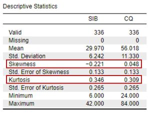
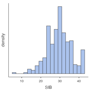
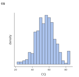
Looking at our results in the preceding images, we see that our skewness and kurtosis values are all within the acceptable range of -2 to +2. Our histograms also confirm that our variables are relatively normally distributed, with approximately symmetrical distributions; however, the way the histograms for each of the variables have a slight tail to the left indicates we may have outliers present in the bottom quartiles of these distributions. To confirm, let’s move to our next assumption.
To report these results in APA format, we can write:
- The scores on both of our study variables were normally distributed, with skewness and kurtosis statistics within the acceptable range of -2 and +2.
Assumption Three: Are there any outliers?
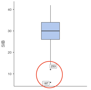
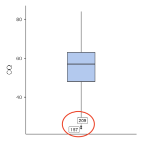
To determine if there are any outliers within any of our study variables, we will look at the boxplot output in the following image. As suspected from the preceding histograms, there are outliers present in the bottom quartiles of both variables. There are two outliers in the Sustainable Innovative Behaviors variable and two outliers present in the Cultural Intelligence variable. As we have discussed before, researchers have to decide whether they are going to keep or delete outliers from their analyses. We will complete our analyses with our outliers for now, but it is good practice to rerun analyses with outliers deleted afterwards to determine if the results of your analyses would be different.
To report this using APA format, we would write:
- There were outliers identified in the bottom quartile of the cultural intelligence and sustainable innovative behaviors distributions, as assessed by an inspection of boxplots. There were two outliers in the sustainable innovative behaviors distribution and two outliers present in the cultural intelligence distribution.
Assumption Four: Are the relationships of interest linear?
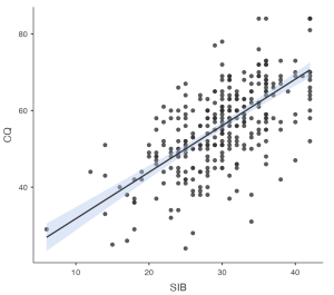
Now we need to look at the scatterplot we requested in our output. Looking at the following scatterplot, our predictor variable (Cultural Intelligence) seems to have a linear relationship with our outcome variable, Sustainable Innovation Behavior.
To report this using APA format, we would write:
- There is a linear relationship between cultural intelligence and sustainable innovative behavior, as visualized using a scatterplot.
Assumption Five: Are there concerns with heteroscedasticity?
Looking back at the preceding scatterplot, there is not a concern for any cone-shaped distributions. Though there is certainly variability along our best-fit line, there is not one area of the line that has drastically different levels of variability than another. In other words, our error variances or residuals seem to be relatively similar across all values of our predictors.
To report this using APA format, we would write:
- There are no concerns regarding heteroscedasticity, after a visual inspection of a scatterplot.
Primary Analyses
Now we are ready to run our linear regression. We can find the regression analysis under the Regression analyses. We will select the option for linear regression from the drop down menu.
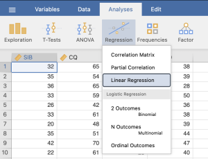
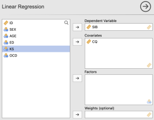
In the main regression menu, we will move over Sustainable Innovation Behavior as our dependent variable and Cultural Intelligence as our covariate (or predictor variable).
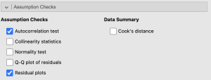
There is nothing we need to adjust in the “model” drop down, so we will move on to “statistics”. In addition to the default settings, we will click:
- Under ‘Assumption Checks’ select:
- ○ Autocorrelation test
- ○ Residual plots
- Under ‘Model Fit’ select:
- ○ Adjusted R²
- ○ RMSE
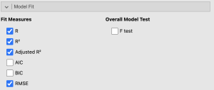
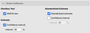
- Under ‘Model Coefficints’ select:
- ○ ANOVA test
- ○ Confidence interval
- ○ Standardized estimate
Now we’re ready to look at our output! First let’s begin by checking our remaining assumption.
Assumption Five: Do we have independence of errors?
One important consideration in regression analysis is whether the residuals (the differences between the actual values and predicted values) are correlated with each other or not. The Durbin-Watson statistic is a measure of this correlation. When the Durbin-Watson statistic is between 1.5 and 2.5, it suggests that there is not a significant correlation between the residuals or errors in our model. This is important because if there is a high degree of correlation between residuals, it can suggest that the model is not capturing all the relevant information about the relationship between the variables. In other words, the model may not be a good fit for the data. A Durbin-Watson statistic outside of the 1.5-2.5 range may indicate that there is a problem with the model, and further investigation may be needed to determine the cause of the correlation between residuals.
The Durbin-Watson statistic is under the Assumption Checks section of your output.
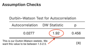
Looking at the preceding figure, we can determine that our Durbin-Watson statistic is within the acceptable range of 1.5-2.5. To report this in APA format:
- The model has acceptable independence of errors, Durbin-Watson = 1.92.
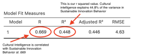
Now that we have finished checking our assumptions, we can move onto the main results. The model fit measures table tells us about the variance explained by our predictor variable, Cultural Intelligence.
Specifically, we want to look at the R and R2 values. The R value is a correlation coefficient that tells us that Cultural Intelligence has a strong, positive correlation with Sustainable Innovation Behavior (r = .669). Looking at our effect size, r2, we can also say that Cultural Intelligence explains 44.8% of the variance in Sustainable Innovation Behavior. Another way of saying that is that 44.8% of the variance in Sustainable Innovation Behavior can be accounted for by Cultural Intelligence.
The next part of the results we will be looking at is the Omnibus ANOVA table. The ANOVA table tells us if our best-fit line explained a big enough portion of variance in the relationship between our variables to be statistically significant. For the variables we have in our model, it is a significant F value because our probability value is smaller than .05 (F = 271, p < .001).
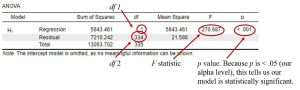
To report this using APA format, we would write:
- Cultural Intelligence significantly predicts Sustainable Innovation Behavior, F (1, 334) = 270.69, p < .001, r2 = .45. Cultural Intelligence explains 44.8% of the variance in Sustainable Innovation Behavior.
Typically, we care more about the individual regression coefficients (slopes) than the overall model significance. To find that information, we move to the last table, labeled model coefficients. In the coefficients table, the first column, labeled Estimate, provides the intercept for the intercept in the first row and the slope for Cultural Intelligence in the second row of output.
We see that our intercept is 9.32, meaning that if a person scored a 0 on CQ, the average Sustainable Innovation Behavior score of that person would be around 9.32. Our slope is .37, meaning that for every one-unit increase in CQ, people are expected to score .37 more on SIB. Putting this together, we could write out our regression equation:
Sustainable Innovation Behavior = .37 (Cultural Intelligence score) + 9.32
We are also given an estimate of error around our slope and intercept in the second column. This error term is used to compute the t value. For example, if you divide the slope by the standard error (.369 / .022) you would get our t value of 16.45. Our t value of 16.45 has an associated p value of < .001. Because this is less than our alpha level (.05), this tells us that the slope is significantly different from zero. This means there is a significant relationship between Cultural Intelligence and Sustainable Innovation Behavior, b = .37, SE = .02, t (334) = 16.45, p < .001. [Note: the df for t is the same as the degree of freedom reported in the residual row on the omnibus ANOVA table.]
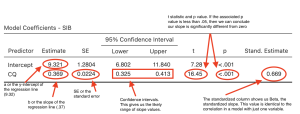
Some additional pieces of output to notice are the standardized estimate and the confidence intervals. The standardized column gives us beta, which is the standardized slope. These values range from 0 to 1, just like a correlation. You may have noticed the standardized slope is the same as our R value in the Model Fit Measures. These values will be the same if you only have one predictor variable. The confidence interval tells us a range of likely slope values within the population. If we sampled 100 times, 95 of those times, we would expect a slope estimate between .33 and .41.
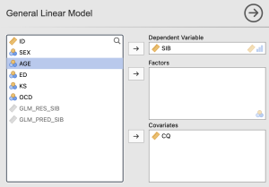
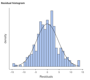
To see a residuals histogram, navigate to the Linear Models analysis button and select ‘General Linear Model’. Use the arrows to move SIB into the Dependent variables box and CQ into the Covariates box as shown below.
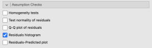
Under Assumption Checks, select “Residuals Histogram”, which will produce the following graph.
Putting it all Together
What do you need to report in your results?
| Value (Notation) | Assumptions |
| slope (b) | Skewness and Kurtosis |
| standard error of slope (SE) | Histogram or Boxplot |
| t value (t) | Scatterplot |
| Degrees of Freedom (df) | VIF/Tolerance |
| Probability (p) | Plot of residuals |
| Effect Size (r2 or R2) |
It’s time to summarize the results of our regression analysis in APA format.
Prior to conducting a simple linear regression, we tested several assumptions. We examined our predictor (Cultural Intelligence) and outcome (Sustainable Innovation Behavior) variables for normality and outliers. Skewness and kurtosis values were all in the normal range and visualizing the variables with boxplots and histograms revealed four outliers that were retained for analysis. Using a scatterplot, we also confirmed a linear relationship between the variables with no evidence of heteroscedasticity. The residual histogram showed the residuals were approximately normally distributed.
For our primary analyses, we examined how Cultural Intelligence predicted Sustainable Innovation Behavior. The overall model was significant, F (1, 334) = 271, p < .001, r2 = .45. There was a significant relationship between Cultural Intelligence and Sustainable Innovation Behavior, b = .37, SE = .02, t (336) = 16.45, p < .001. Our slope is .37, meaning that for every one-unit increase in Cultural Intelligence, people are expected to score .37 higher on Sustainable Innovation Behavior. Cultural Intelligence explained 44.8% of the variance in Sustainable Innovation Behavior.
References
Gölgeci, I., Swiatowiec-Szczepanska, J., & Raczkowski, K. (2017). How does cultural intelligence influence the relationships between potential and realised absorptive capacity and innovativeness? Evidence from Poland. Technology Analysis & Strategic Management, 29(8), 857–871. https://doi.org/10.1080/09537325.2016.1245858
Hu, S., Gu, J., Liu, H. & Huang, Q. (2017). The moderating role of social media usage in the relationship among multicultural experiences, cultural intelligence, and individual creativity. Information Technology & People, 30(2), pp. 265-281. https://doi.org/10.1108/ITP-04-2016- 0099
Li, J., Wu, N., & Xiong, S. (2021). Sustainable innovation in the context of organizational cultural diversity: The role of cultural intelligence and knowledge sharing. PloS One, 16(5), e0250878–e0250878. https://doi.org/10.1371/journal.pone.0250878
Pandey, A. & Charoensukmongkol, P. (2019). Contribution of cultural intelligence to adaptive selling and customer-oriented selling of salespeople at international trade shows: does cultural similarity matter? Journal of Asia Business Studies, 13(1), pp. 79-96. https://doi.org/10.1108/JABS-08-2017-0138
Authors
This guide was written and created by Ruth V. Walker, Ashlyn A. Moraine, Kristen J. Black, Chloe Oberkirch, and Matt C. Cavanaugh. Please address any questions, concerns, or edits to Ruth Walker at ruth-walker@utc.edu
Acknowledgements
We would like to thank Jinlong Li, Na Wu, and Shengxu Xiong for generously publishing their data through PloS One.
Copyright
CC BY-NC-ND: This license allows reusers to copy and distribute the material in any medium or format in unadapted form only, for noncommercial purposes only, and only so long as attribution is given to the creator.