
5
Ashlyn A. Moraine; Erin N. Prince; Ruth V. Walker; Chloe Oberkirch; and Matt C Cavanaugh
Download Data Sets:
The Pew Research Center collected and published survey data on attitudes toward women in leadership as part of their American Trends Panel Survey in 2018. This report detailed the findings from a sample of 4,587 participants who completed an online survey. As part of their report, Parker, Horowitz, and Igielnik (2018) discussed the disparities in attitudes toward women in leadership positions – both in political and corporate settings – by gender, political party, and age. For example, they reported that the majority of women said gender discrimination is a major reason there aren’t more women in high political offices and top executive business positions; however, only 36% of men agreed it was an issue for high political offices and 44% for top executive business positions. When they looked at gender and age together, the majority of women agreed gender discrimination in a barrier to leadership across all ages, while only 35% of men 18-49 years old agreed and 38% of men 50 years and older agreed. We are going to follow up on their analyses by taking a more nuanced look at the interaction between age and gender on attitudes toward women in leadership using their data set – specifically, we are going to focus on women in political positions.
Our first factor, gender, has two levels: (1) woman and (2) man. Our second factor, age, will have three levels: (1) younger adult (30-49 years older), (2) middle-aged adult (50-64 years old), and (3) older adults (65 years and older). Our dependent variable, attitudes toward women in politics, was created by creating an average of participant responses to 23 items that accessed attitudes toward women in political positions. Higher scores on this variable mean more favorable attitudes toward women in politics.
This study utilized a quasi-experimental research design. We do not have a control group and are not randomly assigning participants to a particular gender or age. We are simply grouping participants into the gender they identified with and the age group based on their reported age when the data were collected. The table below shows our 2×3 factorial ANOVA study design.
| Factor Two: Age | |||
| Factor One: Gender | 30-49 years old (Level 1) |
50-64 years old (Level 2) |
65+ years old (Level 3) |
| Women (Level 1) |
30-49 years old, women | 50-64 years old, women | 65+ years old, women |
| Men (Level 2) |
30-49 years old, men | 50-64 years old, men | 65+ years old, men |
Hypotheses
The null hypotheses:
Factor One (Main Effect of Gender)
- Conceptual H0A: There are no significant mean differences in favorable attitudes toward women in politics between women and men.
- Mathematical H0A: There are no significant differences between the population means for women and men on favorable attitudes toward women in politics. M1 = M2
Factor Two (Main Effect of Age Group)
- Conceptual H0B: There are no significant mean differences in favorable attitudes toward women in politics between the three age groups.
- Mathematical H0B: There are no significant differences between the population means for the 30-39 years old group, 50-64 years old group, and 65+ years old group on favorable attitudes toward women in politics. M1 = M2 = M3
Factor One x Factor Two (Interaction between Gender and Age Group)
- Conceptual H0AB: There is not a significant interaction between gender and age on favorable attitudes toward women in politics.
- Mathematical H0AB: Gender x Age Group = 0 for each cell.
The alternative hypotheses:
Factor One (Main Effect of Gender)
- Conceptual H1A: There is a significant mean difference in favorable attitudes toward women in politics between women and men.
- Mathematical H1A: There is a significant difference between the population means for women and men on favorable attitudes toward women in politics. M1 ≠ M2
Factor Two (Main Effect of Age Group)
- Conceptual H1B: There is a significant mean difference in favorable attitudes toward women in politics between the three age groups.
- Mathematical H1B: There is a significant difference between the population means for the 30-39 years old group, 50-64 years old group, and 65+ years old group on favorable attitudes toward women in politics. M1 ≠ M2 ≠ M3
Factor One x Factor Two (Interaction between Gender and Age Group)
- Conceptual H1AB: There is a significant interaction between gender and age on favorable attitudes toward women in politics.
- Mathematical H1AB: Gender x Age Group ≠ 0 for at least one cell.
Jamovi Analyses
In order to run analyses in Jamovi, the first thing we need to do is open the data set we will be working with. To do this, open Jamovi and complete the following steps.
Click on File → Open → Computer → Browse → Choose the Two-Way ANOVA Practice Data (Pew Research Center 2019 W36)
Before we get started with our analyses, we are going to filter our AgeGroup variable to filter out participants who were in the 18-29-year-old age group. Unfortunately, the sample size in this group was too small to compare to the other age groups in this analysis.
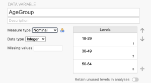
First, navigate to the Data dab and click the Setup button. You can now designate the 4 levels as follows:
- 1 = 18-29; 2 = 30-49; 3 = 50-64; 4 = 65+
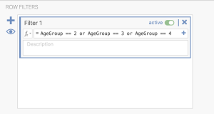
Navigate to the Data tab and click ‘Filters’. In the syntax box, designate that you would like to retain age groups 2, 3, and 4. See image below.
Assumption Testing
Prior to running our two-way ANOVA, we first must check to make sure we meet the assumptions for this statistical test.
Assumption One: Are our factors measured at the categorical (i.e., nominal) level with two or more groups?
Yes. Our independent variables for this study are gender and age. Our first factor, participant gender, had two levels: women and men. Participants who participated in this survey either identified themselves as a woman or a man. Thus, this factor is dichotomous and categorical. If you look at the data label icon in Jamovi, you can see it has the appropriate icon (three overlapping circles) for a nominal/categorical variable. Our second factor, age, had three levels: 30-39 years old, 50-64 years old, and 65+ years old. This factor is categorical and has the appropriate icon in JASP to indicate it is a nominal variable. We meet this assumption.
Assumption Two: Is the dependent variable continuous (i.e., ratio or interval)?
Yes. Our dependent variable for this study is participants’ mean score for their responses to the 23-items measuring their level of favorable attitudes toward women in politics. This variable is continuous, meaning it was measured at the interval or ratio level. If you look at the data label icon in Jamovi, you can see it has the appropriate icon (a ruler) for a scale or continuous variable. We meet this assumption.
Assumption Three: Are the samples independent?
Yes. Looking at our data set, we can determine that the groups of participants in each cell of our research design are independent. In our dataset, you can see that all participants identified as either a woman or a man for factor one. You can also see that participants reported that their age group was one of the following: 30-39 years old, 50-64 years old, and 65+ years old. When we display the levels of both of our factors in a table, as you see below, we have six independent cells representing the possible combinations of our two factors for our 2×3 ANOVA. Thus, knowing the research design did not allow for participants to be exposed to more than one condition or level of either factor, we can conclude that participants in all cells are independent of one another. No participant is in more than one group. We meet this assumption.
| 30-49 years old | 50-64 years old | 65+ years old | |
| Women | Cell 1 Women, 30-49 years | Cell 2 Women, 50-64 years | Cell 3 Women, 65+ years |
| Men | Cell 4 Men, 30-49 years |
Cell 5 Men, 50-64 years |
Cell 6 Men, 65+ years |
Assumption Four: Is the dependent variable normally distributed for each group of the IV?
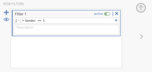
Before we run our descriptive statistics, we have to filter our first factor. To do this, click on “Filters” and type in the variable and value you wish to retain, in our case “Gender = = 1”. This will filter out women participants and allow us to calculate the descriptive statistics for the top row of our 2×3 ANOVA. We do not have to filter out those who refused to respond because we already designated that value as missing and Jamovi will exclude it automatically.
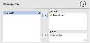
To check our data for the next two assumptions, we will use the Descriptives analysis tab. Click Descriptives. When the “Descriptive Statistics” window pops up, we will need to move our dependent variable to the “Variables” box and our independent variable to the “Split” box using the arrows depicted in the photo below – this is so we can examine normality in the DV for the three levels of our second factor separately.

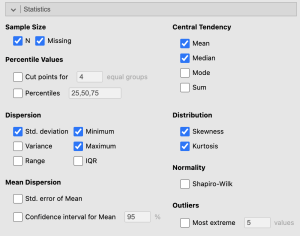
Once we have our variables in the appropriate boxes and our first factor filtered, we are going to ask Jamovi to run the various statistics and graphics we will need to interpret for our assumptions by clicking on the appropriate boxes in the test window. We will be asking Jamovi to provide us with all possible output we may want to look at for our assumptions; however, we will focus on interpreting the output that you will be expected to analyze for your course assignments.
- Under the “Statistics” tab we will check the “Skewness,” and “Kurtosis boxes.”
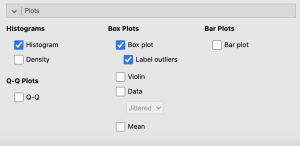
- Under the “Plots” tab we will check “Distribution plots,” “Boxplots,” and “Label outliers” boxes.
See the following image to make sure your test window has all the appropriate boxes selected.
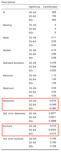
As a reminder, for this course, we will focus on interpreting the skewness and kurtosis statistics to determine if our data are normally distributed. We want our skewness and kurtosis statistics to be between -2 and +2. For this study design, we have six different cells that we have to check to determine if each of those six groups of participants have a normal distribution of attitudes toward women in politics.
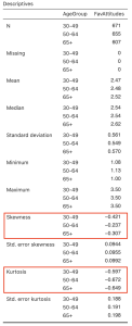
Looking at the values on the output above, we can see our skewness values for the 30-49-year-old group (-0.42), 50-64-year-old group (-0.24), and 65+ group (-0.31) are all within the acceptable range of -2 and +2. Additionally, the kurtosis for the 30-49-year-old group (-0.59), 50-64-year-old group (-0.67), and 65+ group (-0.65) are also within the acceptable range of -2 and +2.
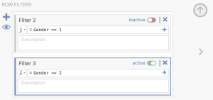
Now that we have analyzed the descriptive statistics for participants in the participants who identified as a man, we have to conduct the same steps for participants who identified as a woman. To do this, click on “Filters.” Next you will toggle your filter for men off and click the blue “+” button to add a third filter. Follow the same formula to retain women. This will filter out participants who identified as men and allow us to calculate the descriptive statistics for the bottom row of our 2×3 ANOVA.
Once this is completed, you will want to repeat the steps above to run Descriptives again with our remaining three groups.
Looking at the values on the output above, we can see our skewness values for the 30-49-year-old group (-0.62), 50-64-year-old group (-0.55), and 65+ group (-0.48) are all within the acceptable range of -2 and +2. Additionally, the kurtosis for the 30-49-year-old group (-0.31), 50-64-year-old group (-0.05), and 65+ group (-0.21) are also within the acceptable range of -2 and +2. The skewness and kurtosis statistics for each of our six cells are also reported in the table below.
| 30-49 years old | 50-64 years old | 65+ years old | |
| Women | Cell 1 Skewness: -0.62 Kurtosis: 0.31 | Cell 2 Skewness: -0.55 Kurtosis: -0.05 | Cell 3 Skewness: -0.48 Kurtosis: -0.21 |
| Men | Cell 4 Skewness: -0.42 Kurtosis: -0.59 |
Cell 5 Skewness: -0.24 Kurtosis: -0.67 |
Cell 6 Skewness: -0.31 Kurtosis: -0.65 |
To report these results in APA format, we could write:
- Attitudes toward women in politics was normally distributed within all six cells, with skewness and kurtosis statistics between -2 and +2.
Now that we have checked our data for normality, let’s take a look at our boxplots for each cell to see if we have outliers in any of our study cells.
Assumption Five: Are there any outliers in the sample?
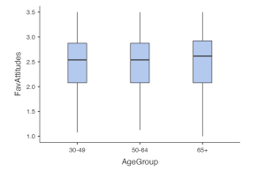
To assess for outliers, we will look at the boxplots in our JASP output. If we have outliers, they would be outside the top and bottom lines or whiskers. When we look at the boxplot for participants who identified as a man, you can see there are no outliers visible in 30-49-year-old age group, 50-64-year-old age group, or the 65+ age group.
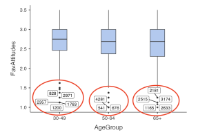
However, if we look at the boxplot for participants who identified as women, you can see we have a lot of outliers across all three age groups, below the lower quartile.
To report this in APA format, we could write:
- There were five outliers in the 65+, women group and several outliers in both the 50-64-year-old, women group and in the 30-49-year-old, women group as assessed by the inspection of a boxplot.
As we discussed in previous chapters, when we have outliers we have to decide if they are going to correct it, keep it, delete it, or replace it. This data has already been checked and cleaned by researchers with the Pew Research Center; thus, we can assume these outliers are not due to a data entry error. As a researcher, you would then have to decide if the outliers are exerting a significant enough impact on your results to warrant deletion. Given that outliers are especially common in datasets with large samples (as ours is; N = 4,337), and that we have so many, we will keep these outliers in our dataset in order to avoid removing a significant amount of data points from our model (something that is generally discouraged, Faraway, 2015). Instead, we will model how to run the analyses as normal with outliers present, and at the end of this chapter, will run the analyses with those outliers removed to examine whether the results remained the same.
Assumption Six: Are there homogeneity of variances?
To determine if we have homogeneity of variances, we need to ask Jamovi to run our two-way ANOVA. Checking for this assumption is a part of the overall two-way ANOVA. Let’s move onto our primary analyses below, and complete checking this assumption in that section.
Primary Analyses
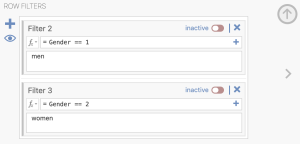
Before running our primary analyses, we need to turn off the filter for Gender. To do this, click on “Filters” and toggle both Gender filters to “inactive”.
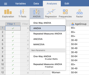
To run a two-way ANOVA, go to ANOVA at the top of the JASP screen and click on ANOVA. See the image below.
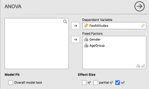
- First, we need to move our dependent variable FavAttitudes to the “Variables” box and our factors Gender and AgeGroup to the “Fixed Factors” box. We are then going to ask Jamovi to run our omnibus test by clicking on the appropriate boxes in the test window.
- Under “Display” we will check the “Descriptive statistics” and “Estimates of effect size” test boxes.
- Under “Estimates of effect size” we will check the omega squared “ω2” box.
See the image below to make sure your test window has all the appropriate boxes selected.
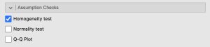
Next, we are going to ask Jamovi to give us the statistics for our final assumption – homogeneity of variances.
4. Under “Assumption Checks” we will check the “Homogeneity tests” box.
Are there homogeneity of variances?
Now that we have asked Jamovi to run our first set of analyses, we can begin our interpretation of the results. The first thing we need to do is go back to our last assumption and determine if we meet the assumption for homogeneity of variances. As you can see from the output below, the p value for our Levene’s test is < .001. Because p is < .05, we can conclude that we do not meet this assumption. If we did not have equal sample sizes in each of our groups, we could potentially conduct a nonparametric test equivalent instead, the Scheirer-Ray-Hare test.
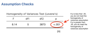
To report the results of the Levene’s test in APA format, it might look something like this:
- There was not homogeneity of variances, as assessed by the Levene’s test for equality of variances (p < .05); however, because there was an approximately equal number of participants in each cell, the two-way ANOVA is considered robust to this violation (Maxwell & Delaney, 2004).
Interpreting the Statistical Significance of Two-Way ANOVAs
Now that we have completed the assumption checking for this statistical test, we can proceed with interpreting the primary analyses. The first thing we will interpret is the statistical significance of the omnibus test results. To do this, we are going to look at the “ANOVA – FavAttitudes” table. We have a total of three different F tests that we will interpret for each of our hypotheses.
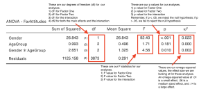
To interpret the results, we want to look at the p values for the main effect for factor one (hypothesis one), the main effect for factor two (hypothesis two), and the interaction (hypothesis three). If p is less than our alpha level of .05, we will reject the null hypothesis.
- There is a significant statistical difference between the group means of our first factor, gender, because p < .001. Because our p value is less than our alpha level of .05, we will reject our first null hypothesis. Thus, we would say we have a main effect of gender on participant attitudes toward women in politics.
- There is not a significant statistical difference between the group means of our second factor, age group, because p = .18. Because our p value is greater than our alpha level of .05, we will fail to reject our second null hypothesis. Thus, we would say we do not have a main effect of age on participant attitudes toward women in politics.
- There is a significant interaction between gender and age group because p = .01. Because our p value is less than our alpha level of .05, we will reject our third null hypothesis. Thus, we would say we do have a significant interaction between gender and age group on participant attitudes toward women in politics.
Writing the basic results of a two-way ANOVA in APA format follows this general format:
- F(df1, df2) = F statistic, p < .05 or > .05, ω2 = omega-squared statistic
However, with a two-way ANOVA, we have three F statistics to report: (1) main effect for our first factor, (2) main effect for our second factor, and (3) our interaction. Plugging our results above into this format, we have:
Main Effect for Factor One: F(1, 3873) = 92.39, p < .001, ω2 = .02
Main Effect for Factor Two: F(2, 3873) = 1.71, p > .05, ω2 = .00
Main Effect for the Interaction: F(2, 3873) = 4.56, p < .05, ω2 = .002
Now we know that we have a significant interaction between our two factors – gender and age group – but what does that mean? To answer this, we are going to do two things: (1) graph the means of each cell in our interaction to help us visualize what is happening with the data and (2) conduct post hoc tests called simple main effects.
We can graph the means of the interaction using Jamovi or using Excel. For now, let’s take the easy way out and ask Jamovi to provide us with a graph of the interaction.
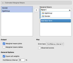
- In the ANOVA analysis window, click on “Estimated Marginal Means” dropdown.
- Click the blue “Add New Term” button.
- Press down the Shift button on your keyboard and select “AgeGroup” then “Gender.
- Make sure to select the variables in this order otherwise your graph will show three lines instead of two.
- Once you have both variables selected, move them into the “Marginal Means” box with the arrow button.
Let’s take a look at the group means plotted on the following graph:
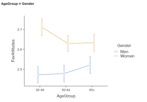
Looking at the Descriptive plots or line graph above, we can see that we have an ordinal interaction – the group means do not cross or overlap in our graph. By graphing the means of each of our study cells, we can visualize what is happening with our data.
For example, looking at this graph we can see women in the younger (30-49-year-old) age group reported the most favorable attitudes toward women in politics. Alternately, men in the younger age group reported the least favorable attitudes toward women in politics. This graph is limited because it does not tell us which groups are significantly different from one another. However, by asking Jamovi to display error bars using the confidence intervals, we are able to take an educated guess as to where the statistical differences will be.
The dots on the graph indicate the group means and the error bars indicate the 95% confidence intervals around the means. A general indication of how spread out or variable participant ratings of attitudes toward women in politics were in each group. Groups that do not have overlapping error bars are more likely to be significantly different from one another; however, this is not guaranteed – so post hoc tests are needed to confirm. Looking at the line graph above, it seems likely that women across all age groups had significantly more favorable attitudes toward women in politics than men.
The group with the smallest gender differences in attitudes toward women in politics was the older adult age group. To confirm our interpretation of the graph is correct, we will conduct post hoc tests. A commonly used post hoc test to help interpret significant interactions with two-way ANOVAs are simple main effects.
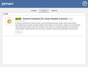
Our next step is to run tests of simple effects. Within the ANOVA menus that are part of the base Jamovi program, simple effects are not currently an option that can be requested (as at v. 1.6.12). However, Jamovi has a range of add-on modules that can be activated which expand the analysis options available. One of these, the General Analyses for Linear Models in Jamovi, or gamlj module, will allow us to obtain our simple effects.
To add this package, click the blue plus sign labeled “Modules” in the top right corner of the Jamovi window.

From the dropdown menu, select “Jamovi Library.”
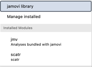
A window will appear, type “gamlj” in the search bar and click “Install” once you see this result.
Once you have installed the gamlj package, this new Linear Models option should appear in your analyses tab.

To perform our Simple Effects analysis, click on Linear Models, selecting “General Linear Model” from the dropdown menu. You will see a menu that looks similar to the set up menu for our ANOVA analysis. Simply set these variables up the same way we did for our ANOVA analysis.
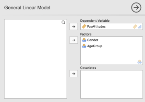
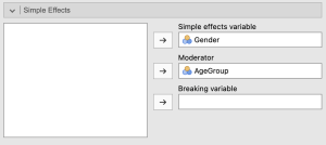
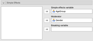
Scroll down to the Simple Effects menu in the General Linear Model window. Using the arrow buttons, move “Gender” into the “Simple effects variable” box and “AgeGroup” into the “Moderator” box.
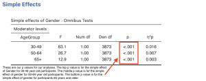
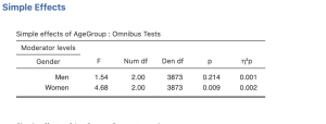
The results of the additional simple main effects analyses are copied below:
Repeat this process but with “AgeGroup” in the “Simple effects variable” box and “Gender” in the “Moderator” box.
This will test to see if there are differences in our second factor, age group, at each level of the first factor (women, men). Our results are copied below.
To interpret simple effects, we will focus on the p values for each comparison.
- The p value on top (p < .001), tells us that when we compare attitudes toward women in politics for women and men who are 30-49 years old, there is a significant difference because p is less than .05.
- The p value in the middle (p < .001), tells us that when we compare attitudes toward women in politics for women and men who are 50-64 years old, there is a significant difference because p is less than .05.
- The p value on the bottom (p < .001), tells us that when we compare attitudes toward women in politics for women and men who are 65 years and older, there is a significant difference because p is less than .05.
To report the results of our simple main effects analyses, we could write:
- After conducting analyses of simple main effects, we found a significant difference in attitudes toward women in politics between women and men across in the younger adult (F(1) = 63.14, p < .001), middle-aged adult (F(1) = 26.75, p < .001), and older adult age groups (F(1) = 12.94, p < .001). Across all age groups, women had significantly more favorable views toward women in politics compared to men. Further, there was not a simple main effect of age for men, F(2) = 1.54, p > .05. There were no differences in attitudes toward women in politics across age groups for men. However, there was a simple main effect of age for women, F(2) = 4.68, p < .01. Younger women held more favorable attitudes toward women in politics than the middle-aged and older age groups.
Interpreting the Practical Significance of Two-Way ANOVAs
Now that we have interpreted the statistical significance, we will look at the practical significance by looking at our effect size. A significant p value tells us that there is a significant interaction between gender and age on attitudes toward women in politics, but the effect size tells us how much of our dependent variable we are explaining with these factors.
Reminder: Omega Squared Effect Sizes (Cohen, 1988; Kirk, 1996)
| Effect Size | Strength |
| .01 | Small |
| .06 | Medium |
| .14 | Large |
We obtained an omega-squared value of .002 for our interaction, this is less than a small effect. There is a statistical interaction between gender and age on attitudes toward women in politics, but the variance explained by that interaction is very small. Meaning, the interaction between gender and age only explains .2% of the variance in participant attitudes toward women in politics. If we look at our main effect for gender, however, the omega-squared value was .02. This means that the variance in participant attitudes toward women in politics explained by gender alone was 2.3%, still a small amount, but larger than the interaction.
Reporting in APA Format
What do you need to report in your results?
| Value (Notation) | ||
| Means (M) | Standard Deviations (SD) | Test Statistics (F) |
| Degrees of Freedom (df) | Probabilities (p) | ω2 or η2 |
| Confidence Intervals | Assumptions | Skewness and Kurtosis |
| Boxplot | Levene’s Statistic | Post Hoc Test |
| Simple Main Effect | Effect Size |
Putting it All Together
Now, let’s write up the results of our test combining everything we’ve done so far, including the test of assumptions, and the results of the two-way ANOVA.
A two-way ANOVA was conducted to determine if there was an interaction between gender and age on attitudes toward women in politics. Attitudes toward women in politics was normally distributed within all six cells, with skewness and kurtosis statistics between -2 and +2. There were five outliers in the 65+, women group; 19 outliers in the 50-64-year-old, women group; and 21 outliers in the 30-49-year-old, women group as assessed by the inspection of a boxplot. There was not homogeneity of variances, as assessed by the Levene’s test for equality of variances (p < .05); however, because there was an approximately equal number of participants in each cell, the two-way ANOVA is considered robust to this violation (Maxwell & Delaney, 2004).
There was a statistically significant interaction between gender and age on attitudes toward women in politics, F(2, 3873) = 4.56, p < .05, ω2 = .002. There was also a main effect of gender on attitudes toward women in politics, F(1, 3873) = 92.39, p < .001, ω2 = .02. There was not a main effect of age group, F(2, 3873) = 1.71, p > .05, ω2 = .00. After conducting analyses of simple main effects, we found a significant difference in attitudes toward women in politics between women and men across in the younger adult (F(1) = 63.14, p < .001), middle-aged adult (F(1) = 26.75, p < .001), and older adult age groups (F(1) = 12.94, p < .001). Across all age groups, women had significantly more favorable views toward women in politics compared to men. Further, there was not a simple main effect of age for men, F(2) = 1.54, p > .05. There were no differences in attitudes toward women in politics across age groups for men. However, there was a simple main effect of age for women, F(2) = 4.68, p < .01. Younger women held more favorable attitudes toward women in politics than the middle-aged and older age groups.
Real World Meaning
Remember, when we interpret the real world meaning of a study, we want to take out any statistical jargon and describe the results of the study in a way that is easy to understand by people who do not know anything about statistics. Think about how you would describe the results to your roommate, sibling, parent, or neighbor. For example, if I was telling my neighbor the real world meaning of our results, I would say:
- When researchers studied the impact of gender and age on attitudes toward women in politics they found a few things: (1) men have less favorable attitudes toward women in politics across all age groups, (2) there are differences in attitudes toward women in politics between young, middle-aged, and older women – but not between different ages for men, and (3) younger women have the most favorable attitudes toward women in politics. In fact, younger women had more favorable attitudes toward women in politics compared to all of the men in the study, and more favorable attitudes compared to the middle-aged and older women as well.
References
Parker, K., Horowitz, J., & Pumphrey, J. (2018). Women and leadership 2018. Pew Research Center. Retrieved from https://www.pewresearch.org/social-trends/wp-content/uploads/sites/3/2018/09/Gender-and-leadership-for-PDF_updated-10.1.pdf
Authors
This guide was written and created by Ruth V. Walker, PhD, Ashlyn A. Moraine, Chloe Oberkirch, Matt C. Cavanaugh, and Erin N. Prince. Please address any questions, concerns, or edits to Ruth Walker at ruth-walker@utc.edu
Acknowledgements
We would like to thank the Pew Research Center for generously making their data available for secondary analysis. Additionally, we appreciate Dr. Kristen Black’s edits and suggestions during the creation of this guide.
Copyright
CC BY-NC-ND: This license allows reusers to copy and distribute the material in any medium or format in unadapted form only, for noncommercial purposes only, and only so long as attribution is given to the creator.